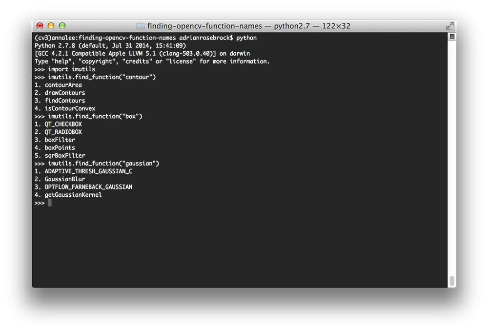
Quantcast
Channel: Tutorials Archives - PyImageSearch
Viewing all 432 articles
Browse latest View live

The perfect computer vision environment: PyCharm, OpenCV, and Python virtual environments

$
0
0

pycharm_opencv_logos

You know what makes for a (not so) fun weekend?

Reconfiguring and reinstalling OSX on your MacBook Pro. Apparently, the 13in MacBook Pro that I use when I’m traveling decided to shit the bed.

No worries though, I use Carbon Copy Cloner and Backblaze, so no data was lost. And to be honest, I was considering rebuilding the development environment on my travel system for awhile now. While I use my 13in MacBook Pro while I travel, I have a second MacBook Pro that I use on a daily basis as my main development system. And over the past two years the development environments between the two have become horribly out of sync and almost unusable.

As I sat down Sunday night, looking out at the anvil-shaped thunderclouds rolling in across the Long Island sound, I took a second and sipped some tea (spiked with some peppermint schnapps; it is the weekend, of course) from my mug and watched as the lighting danced haphazardly across the sky.

There is a certain calming serenity that comes with watching a thunderstorm roll in — and hopefully the rest of this guide gives you some calming serenity yourself when you go to setup PyCharm to play nice with OpenCV and virtual environments.

PyCharm, virtual environments, and OpenCV

The rest of this blog post will assume that you have already installed OpenCV and the appropriate Python bindings on your system. I’m also going to assume that you have virtualenv and virtualenvwrapper installed as well.

These installation instructions and associated screenshots were gathered on my OSX machine, but these instructions will work on both Linux and Windows (for Windows you’ll have to change the various paths to files of course, but that’s okay).

I’ll also be setting up my system with Python 2.7 and OpenCV 2.4.X; however, you can use the same instructions to setup your environment with Python 3 and OpenCV as well, you’ll just need to change the paths to the Python and OpenCV files.

Step 1: Create your virtual environment

The first thing we are going to do is setup our virtual environment. Open up a terminal and create your virtual environment. For this example, let’s name the virtual environment

pyimagesearch
 :
$ mkvirtualenv pyimagesearch

Now that our virtual environment has been setup, let’s install NumPy, Scipy, matplotlib, scikit-learn, and scikit-image which are all commonly used for computer vision development:

$ pip install numpy
$ pip install scipy
$ pip install matplotlib
$ pip install scikit-learn
$ pip install -U scikit-image

Step 2: Sym-link your cv2.so and cv.py files

As I’m sure you already know, OpenCV is not pip-installable. You’ll need to manually sym-link your

cv2.so
  and
cv.py
  files into the site-packages directory of the
pyimagesearch
  virtual environment.

On my system, OpenCV is installed in 

/usr/local/lib/python2.7/site-packages/

This may not be the case for your system, so be sure to find your OpenCV install path and make note of it — you’ll need this path for the following step.

Now that we have the path to our OpenCV install, we can sym-link it into our virtual environment:

$ cd ~/.virtualenvs/pyimagesearch/lib/python2.7/site-packages/
$ ln -s /usr/local/lib/python2.7/site-packages/cv.py cv.py
$ ln -s /usr/local/lib/python2.7/site-packages/cv2.so cv2.so

Step 3: Configure PyCharm

If you are not already using the PyCharm IDE for editing your code, it’s definitely worth a look. They have both a free community edition and a paid version with a bunch of nice bells and whistles.

It’s hard to believe, but for years I turned the other way at PyCharm and dismissed it.

You see, back in college I was forced to use Eclipse for Java development — and since I was never fond of Java or Eclipse, I (ignorantly) turned my back on any IDE that reminded me of it. Boy, that was a huge mistake.

About six months ago I decided to give PyCharm a real chance and not let my previous experiences bias my opinion. In short, it was one of the best choices I’ve ever made in terms of development environments.

Anyway, now that our virtual environment is all setup let’s connect it to a PyCharm project.

Open up PyCharm and create a new “Pure Python” project:

Creating a new Pure Python project in PyCharm.

Figure 1: Creating a new Pure Python project in PyCharm.


From here we need to set the location of our Python Interpreter. In most cases this location will point to your system install of Python. However, we do not want to use the system Python — we want to use the Python that is part of our

pyimagesearch
  virtual environment, so click the gear icon and select “Add Local”:
Figure 2: Specifying that we want to use a local Python environment rather than the default system Python.

Figure 2: Specifying that we want to use a local Python environment rather than the default system Python.

Next up, we need to specify the path to the Python binary inside our virtual environment.

In my case, the

pyimagesearch
  virtual environment is located in 
~/.virtualenvs/pyimagesearch/
 with the actual Python binary in 
~/.virtualenvs/pyimagesearch/bin
 .

In any case, be sure to navigate to the Python binary for your virtual environment, followed by clicking “Choose”:

Figure 3: Selecting the pyimagesearch Python binary.

Figure 3: Selecting the pyimagesearch Python binary.

After you have selected your virtual environment, PyCharm will spend a few seconds updating the project skeletons:

Figure 4: PyCharm updating the project skeletons for our computer vision virtual environment.

Figure 4: PyCharm updating the project skeletons for our computer vision virtual environment.

Once the skeletons are done updating, click the “Create” button to launch your project.

And that’s all there is to it!

Done!

After this, you’re all set. PyCharm will use your

pyimagesearch
  virtual environment and will recognize the OpenCV library.

And if you ever want to update the virtual environment for a project you are using, just to the PyCharm Preferences panel, select the Project tab on the left sidebar, followed by “Project Interpreter”:

Figure 5: Updating the virtual environment for a project already created with PyCharm.

Figure 5: Updating the virtual environment for a project already created with PyCharm.

Summary

In this blog post I showed you how to utilize virtual environments and OpenCV inside my favorite IDE, PyCharm.

I hope you find this post useful when you go to setup your next Python + OpenCV project!

And if you aren’t using PyCharm yet, it’s definitely worth a look.

The post The perfect computer vision environment: PyCharm, OpenCV, and Python virtual environments appeared first on PyImageSearch.


How to find functions by name in OpenCV

$
0
0

opencv_func_names_examples

OpenCV can be a big, hard to navigate library, especially if you are just getting started learning computer vision and image processing.

The release of OpenCV 3 has only further complicated matters, moving a few important functions around and even slightly altering their names (the

cv2.cv.BoxPoints
  vs.
cv2.boxPoints
  methods come to mind off the top of my head).

While a good IDE can help you search and find a particular function based on only a few keystrokes, sometimes you won’t have access to your IDE. And if you’re trying to develop code that is compatible with both OpenCV 2.4 and OpenCV 3, then you’ll need to programmatically determine if a given function is available (whether via version detection or function listing).

Enter the

find_function
  method, now part of the imutils library, that can help you search and lookup OpenCV methods simply by providing a query string.

In the rest of this blog post I’ll show you how to quickly and programmatically search and lookup functions in the OpenCV library using only simple Python methods.

Looking for the source code to this post?
Jump right to the downloads section.

Dumping all OpenCV function names and attributes

A quick way to view all OpenCV functions and attributes exposed to the Python bindings is to use the built-in Python 

dir
  function, which is used to return a list of names in the current local scope.

Assuming you have OpenCV installed and a Python shell ready, we can use the

dir
  method to create a list of all OpenCV methods and attributes available to us:
>>> import cv2
>>> funcs = dir(cv2)
>>> for f in funcs:
...     print(f)
... 
ACCESS_FAST
ACCESS_MASK
ACCESS_READ
ACCESS_RW
ACCESS_WRITE
ADAPTIVE_THRESH_GAUSSIAN_C
ADAPTIVE_THRESH_MEAN_C
AGAST_FEATURE_DETECTOR_AGAST_5_8
AGAST_FEATURE_DETECTOR_AGAST_7_12D
AGAST_FEATURE_DETECTOR_AGAST_7_12S
AGAST_FEATURE_DETECTOR_NONMAX_SUPPRESSION
AGAST_FEATURE_DETECTOR_OAST_9_16
AGAST_FEATURE_DETECTOR_THRESHOLD
AKAZE_DESCRIPTOR_KAZE
AKAZE_DESCRIPTOR_KAZE_UPRIGHT
AKAZE_DESCRIPTOR_MLDB
AKAZE_DESCRIPTOR_MLDB_UPRIGHT
AKAZE_create
...
waitKey
warpAffine
warpPerspective
watershed
xfeatures2d
ximgproc
xphoto

While this method does indeed give us the list of attributes and functions inside OpenCV, it requires a manual scan or a grep of the list to find a particular function.

Personally, I like to use this raw list of method names if I have a rough idea of what you’re looking for (kind of like a “I’ll know it when I see it” type of situation); otherwise, I look to use the

find_function
  method of
imutils
  to quickly narrow down the search space — similar to grep’ing the output of
dir(cv2)
 .

Searching the OpenCV library for (partial) function names

Let’s start off this section by defining our

find_function
  method:
# import the necessary packages
from __future__ import print_function
import cv2
import re

def find_function(name, pretty_print=True, module=None):
	# if the module is None, initialize it to to the root `cv2`
	# library
	if module is None:
		module = cv2

	# grab all function names that contain `name` from the module
	p = ".*{}.*".format(name)
	filtered = filter(lambda x: re.search(p, x, re.IGNORECASE), dir(module))
	
	# check to see if the filtered names should be returned to the
	# calling function
	if not pretty_print:
		return filtered

	# otherwise, loop over the function names and print them
	for (i, funcName) in enumerate(filtered):
		print("{}. {}".format(i + 1, funcName))

if __name__ == "__main__":
	find_function("blur")

Lines 2-4 start off by importing our necessary packages. We’ll need

cv2
  for our OpenCV bindings and
re
  for Python’s built-in regular expression functionality.

We define our

find_function
  method on Line 6. This method requires a single required argument, the (partial)
name
  of the function we want to search
cv2
  for. We’ll also accept two optional arguments:
pretty_print
  which is a boolean indicating whether the results should be returned as a list or neatly formatted to our console; and
module
  which is the root-module or sub-module of the OpenCV library.

We’ll initialize

module
  to be
cv2
 , the root-module, but we could also pass in a sub-module such as
xfeatures2d
 . In either case, the
module
  will be searched for partial function/attribute matches to
name
 .

The actual search takes place on Lines 13 and 14 where we apply a regular expression to determine if any attribute/function name inside of

module
  contains the supplied
name
 .

Lines 18 and 19 make a check to see if we should return the list of

filtered
  functions to the calling function; otherwise, we loop over the function names and print them to our console (Lines 22 and 23).

Finally, Line 26 takes our

find_function
  method for a test drive by searching for functions containing the
blur
  in their name.

To see our

find_function
  method in action, just open a terminal and execute the following command:
$ python find_function.py
1. GaussianBlur
2. blur
3. medianBlur

As our output shows, it seems there are three functions inside of OpenCV that contain the text

blur
 , including
cv2.GaussianBlur
 ,
cv2.blur
 , and
cv2.medianBlur
 .

A real-world example of finding OpenCV functions by name

As I already mentioned earlier in this post, the

find_functions
  method is already part of the imutils library. You can install
imutils
  via
pip
 :
$ pip install imutils

If you already have

imutils
  installed on your system, be sure to upgrade it to the latest version:
$ pip install --upgrade imutils

Our goal in this project is to write a Python script to detect the hardcopy edition of Practical Python and OpenCV + Case Studies (which is set to be released on Wednesday, August 16th at 12:00 EST, so be sure to mark your calendars!) in an image and draw a its bounding contour surrounding it:

Our goal is to find the outline (i.e. contours) of the original book (left) and then draw the outline on the book (right).

Figure 1: Our goal is to find the original book in the image (left) and then draw the outline on the book (right).

Open up a new file, name it

find_book.py
 , and let’s get coding:
# import the necessary packages
import numpy as np
import cv2

# load the image containing the book
image = cv2.imread("ppao_hardcopy.png")
orig = image.copy()

# convert the image to grayscale, threshold it, and then perform a
# series of erosions and dilations to remove small blobs from the
# image
gray = cv2.cvtColor(image, cv2.COLOR_BGR2GRAY)
thresh = cv2.threshold(gray, 40, 255, cv2.THRESH_BINARY)[1]
thresh = cv2.erode(thresh, None, iterations=2)
thresh = cv2.dilate(thresh, None, iterations=2)

We start off by loading our image from disk on Line 6. We then do some basic image processing on Lines 12-15, including conversion to grayscale, thresholding, and a series of erosions and dilations to remove any small blobs from the thresholded image. Our output thresholded image looks like this:

Figure 3: The thresholded, binary representation of the book image.

Figure 3: The thresholded, binary representation of the book image.

However, in order to draw the contour surrounding the book, I first need to find the outline of the book itself.

Let’s pretend that I’m stuck and I don’t know what the name of the function is that finds the outline of an object in an image — but I do recall that “outlines” are called “contours” in OpenCV.

By firing up a shell and using the

find_function
  in
imutils
 , I quickly ascertain that that I am looking for the
cv2.findContours
  function:
$ python
>>> import imutils
>>> imutils.find_function("contour")
1. contourArea
2. drawContours
3. findContours
4. isContourConvex

Now that I know I am using the

cv2.findContours
  method, I need to figure out what contour extraction flag should be used for the function. I only want to return external contours (i.e the outer-most outlines) so I’ll need to look up that attribute as well:
>>> imutils.find_function("external")
1. RETR_EXTERNAL

Got it. I need to use the

cv2.RETR_EXTERNAL
  flag. Now that I have that settled, I can finish up my Python script:
# import the necessary packages
import numpy as np
import cv2

# load the image containing the book
image = cv2.imread("ppao_hardcopy.png")
orig = image.copy()

# convert the image to grayscale, threshold it, and then perform a
# series of erosions and dilations to remove small blobs from the
# image
gray = cv2.cvtColor(image, cv2.COLOR_BGR2GRAY)
thresh = cv2.threshold(gray, 40, 255, cv2.THRESH_BINARY)[1]
thresh = cv2.erode(thresh, None, iterations=2)
thresh = cv2.dilate(thresh, None, iterations=2)

# find contours in the thresholded image, keeping only the largest
# one
(_, cnts, _) = cv2.findContours(thresh.copy(), cv2.RETR_EXTERNAL,
	cv2.CHAIN_APPROX_SIMPLE)
c = max(cnts, key=cv2.contourArea)
cv2.drawContours(image, [c], -1, (0, 255, 255), 3)

# show the output image
thresh = np.dstack([thresh] * 3)
cv2.imshow("Output", np.hstack([orig, thresh, image]))
cv2.waitKey(0)

Lines 19 and 20 makes a call to

cv2.findContours
  to find the external outlines of the objects (thanks to the
cv2.RETR_EXTERNAL
  attribute) in the thresholded image.

We’ll then take the largest contour found (which is presumed to be the outline of the book) and draw the outline on our image (Lines 21 and 22).

Finally, Lines 25-27 show our output images.

To see my script in action, I just fire up a terminal and issue the following command:

$ python find_book.py

Figure 2: Our original input image (left), the thresholded, binary representation of the image (center), and the contour drawn surrounding the book (right).

Figure 3: Our original input image (left), the thresholded, binary representation of the image (center), and the contour drawn surrounding the book (right).

Sure enough, we’ve been able to detect and draw the outline of the book without a problem!

Summary

In this blog post we learned how to get the names of all functions and attributes in OpenCV that are exposed to the Python bindings.

We then built a Python function to programmatically search these function/attribute names via a text query. This function has been included in the imutils package.

Finally, we explored how OpenCV function filtering can be used in your every-day workflow to increase productivity and facilitate quick function lookup. We demonstrated this by building a small Python script detect the presence of a book in an image.

Downloads:

If you would like to download the code and images used in this post, please enter your email address in the form below. Not only will you get a .zip of the code, I’ll also send you a FREE 11-page Resource Guide on Computer Vision and Image Search Engines, including exclusive techniques that I don’t post on this blog! Sound good? If so, enter your email address and I’ll send you the code immediately!

The post How to find functions by name in OpenCV appeared first on PyImageSearch.

Blur detection with OpenCV

$
0
0

detecting_blur_header

Between myself and my father, Jemma, the super-sweet, hyper-active, extra-loving family beagle may be the most photographed dog of all time. Since we got her as a 8-week old puppy, to now, just under three years later, we have accumulated over 6,000+ photos of the dog.

Excessive?

Perhaps. But I love dogs. A lot. Especially beagles. So it should come as no surprise that as a dog owner, I spend a lot of time playing tug-of-war with Jemma’s favorite toys, rolling around on the kitchen floor with her as we roughhouse, and yes, snapping tons of photos of her with my iPhone.

Over this past weekend I sat down and tried to organize the massive amount of photos in iPhoto. Not only was it a huge undertaking, I started to notice a pattern fairly quickly — there were lots of photos with excessive amounts of blurring.

Whether due to sub-par photography skills, trying to keep up with super-active Jemma as she ran around the room, or her spazzing out right as I was about to take the perfect shot, many photos contained a decent amount of blurring.

Now, for the average person I suppose they would have just deleted these blurry photos (or at least moved them to a separate folder) — but as a computer vision scientist, that wasn’t going to happen.

Instead, I opened up an editor and coded up a quick Python script to perform blur detection with OpenCV.

In the rest of this blog post, I’ll show you how to compute the amount of blur in an image using OpenCV, Python, and the Laplacian operator. By the end of this post, you’ll be able to apply the variance of the Laplacian method to your own photos to detect the amount of blurring.

Looking for the source code to this post?
Jump right to the downloads section.

Variance of the Laplacian

Figure 2: Convolving the input image with the Laplacian operator.

Figure 1: Convolving the input image with the Laplacian operator.

My first stop when figuring out how to detect the amount of blur in an image was to read through the excellent survey work, Analysis of focus measure operators for shape-from-focus [2013 Pertuz et al]. Inside their paper, Pertuz et al. reviews nearly 36 different methods to estimate the focus measure of an image.

If you have any background in signal processing, the first method to consider would be computing the Fast Fourier Transform of the image and then examining the distribution of low and high frequencies — if there are a low amount of high frequencies, then the image can be considered blurry. However, defining what is a low number of high frequencies and what is a high number of high frequencies can be quite problematic, often leading to sub-par results.

Instead, wouldn’t it be nice if we could just compute a single floating point value to represent how blurry a given image is?

Pertuz et al. reviews many methods to compute this “blurryness metric”, some of them simple and straightforward using just basic grayscale pixel intensity statistics, others more advanced and feature-based, evaluating the Local Binary Patterns of an image.

After a quick scan of the paper, I came to the implementation that I was looking for: variation of the Laplacian by Pech-Pacheco et al. in their 2000 ICPR paper, Diatom autofocusing in brightfield microscopy: a comparative study.

The method is simple. Straightforward. Has sound reasoning. And can be implemented in only a single line of code:

cv2.Laplacian(image, cv2.CV_64F).var()

You simply take a single channel of an image (presumably grayscale) and convolve it with the following 3 x 3 kernel:

Figure 2: The Laplacian kernel.

Figure 2: The Laplacian kernel.

And then take the variance (i.e. standard deviation squared) of the response.

If the variance falls below a pre-defined threshold, then the image is considered blurry; otherwise, the image is not blurry.

The reason this method works is due to the definition of the Laplacian operator itself, which is used to measure the 2nd derivative of an image. The Laplacian highlights regions of an image containing rapid intensity changes, much like the Sobel and Scharr operators. And, just like these operators, the Laplacian is often used for edge detection. The assumption here is that if an image contains high variance then there is a wide spread of responses, both edge-like and non-edge like, representative of a normal, in-focus image. But if there is very low variance, then there is a tiny spread of responses, indicating there are very little edges in the image. As we know, the more an image is blurred, the less edges there are.

Obviously the trick here is setting the correct threshold which can be quite domain dependent. Too low of a threshold and you’ll incorrectly mark images as blurry when they are not. Too high of a threshold then images that are actually blurry will not be marked as blurry. This method tends to work best in environments where you can compute an acceptable focus measure range and then detect outliers.

Detecting the amount of blur in an image

So now that we’ve reviewed the the method we are going to use to compute a single metric to represent how “blurry” a given image is, let’s take a look at our dataset of the following 12 images:

Figure 3: Our dataset of images. Some are blurry, some are not. Our goal is to perform blur detection with OpenCV and mark the images as such.

Figure 3: Our dataset of images. Some are blurry, some are not. Our goal is to perform blur detection with OpenCV and mark the images as such.

As you can see, some images are blurry, some images are not. Our goal here is to correctly mark each image as blurry or non-blurry.

With that said, open up a new file, name it

detect_blur.py
 , and let’s get coding:
# import the necessary packages
from imutils import paths
import argparse
import cv2

def variance_of_laplacian(image):
	# compute the Laplacian of the image and then return the focus
	# measure, which is simply the variance of the Laplacian
	return cv2.Laplacian(image, cv2.CV_64F).var()

# construct the argument parse and parse the arguments
ap = argparse.ArgumentParser()
ap.add_argument("-i", "--images", required=True,
	help="path to input directory of images")
ap.add_argument("-t", "--threshold", type=float, default=100.0,
	help="focus measures that fall below this value will be considered 'blurry'")
args = vars(ap.parse_args())

We start off by importing our necessary packages on Lines 2-4. If you don’t already have my imutils package on your machine, you’ll want to install it now:

$ pip intall imutils

From there, we’ll define our

variance_of_laplacian
  function on Line 6. This method will take only a single argument the
image
  (presumed to be a single channel, such as a grayscale image) that we want to compute the focus measure for. From there, Line 9 simply convolves the
image
  with the 3 x 3 Laplacian operator and returns the variance.

Lines 12-17 handle parsing our command line arguments. The first switch we’ll need is

--images
 , the path to the directory containing our dataset of images we want to test for blurryness.

We’ll also define an optional argument

--thresh
 , which is the threshold we’ll use for the blurry test. If the focus measure for a given image falls below this threshold, we’ll mark the image as blurry. It’s important to note that you’ll likely have to tune this value for your own dataset of images. A value of
100
  seemed to work well for my dataset, but this value is quite subjective to the contents of the image(s), so you’ll need to play with this value yourself to obtain optimal results.

Believe it or not, the hard part is done! We just need to write a bit of code to load the image from disk, compute the variance of the Laplacian, and then mark the image as blurry or non-blurry:

# import the necessary packages
from imutils import paths
import argparse
import cv2

def variance_of_laplacian(image):
	# compute the Laplacian of the image and then return the focus
	# measure, which is simply the variance of the Laplacian
	return cv2.Laplacian(image, cv2.CV_64F).var()

# construct the argument parse and parse the arguments
ap = argparse.ArgumentParser()
ap.add_argument("-i", "--images", required=True,
	help="path to input directory of images")
ap.add_argument("-t", "--threshold", type=float, default=100.0,
	help="focus measures that fall below this value will be considered 'blurry'")
args = vars(ap.parse_args())

# loop over the input images
for imagePath in paths.list_images(args["images"]):
	# load the image, convert it to grayscale, and compute the
	# focus measure of the image using the Variance of Laplacian
	# method
	image = cv2.imread(imagePath)
	gray = cv2.cvtColor(image, cv2.COLOR_BGR2GRAY)
	fm = variance_of_laplacian(gray)
	text = "Not Blurry"

	# if the focus measure is less than the supplied threshold,
	# then the image should be considered "blurry"
	if fm < args["threshold"]:
		text = "Blurry"

	# show the image
	cv2.putText(image, "{}: {:.2f}".format(text, fm), (10, 30),
		cv2.FONT_HERSHEY_SIMPLEX, 0.8, (0, 0, 255), 3)
	cv2.imshow("Image", image)
	key = cv2.waitKey(0)

We start looping over our directory of images on Line 20. For each of these images we’ll load it from disk, convert it to grayscale, and then apply blur detection using OpenCV (Lines 24-27).

In the case that the focus measure exceeds the threshold supplied a command line argument, we’ll mark the image as “blurry”.

Finally, Lines 35-38 write the

text
  and computed focus measure to the image and display the result to our screen.

Applying blur detection with OpenCV

Now that we have

detect_blur.py
  script coded up, let’s give it a shot. Open up a shell and issue the following command:
$ python detect_blur.py --images images

Figure 4: Correctly marking the image as "blurry".

Figure 4: Correctly marking the image as “blurry”.

The focus measure of this image is 83.17, falling below our threshold of 100; thus, we correctly mark this image as blurry.

Figure 5: Performing blur detection with OpenCV. This image is marked as "blurry".

Figure 5: Performing blur detection with OpenCV. This image is marked as “blurry”.

This image has a focus measure of 64.25, also causing us to mark it as “blurry”.

Figure 6: Marking an image as "non-blurry".

Figure 6: Marking an image as “non-blurry”.

Figure 6 has a very high focus measure score at 1004.14 — orders of magnitude higher than the previous two figures. This image is clearly non-blurry and in-focus.

Figure 7: Applying blur detection with OpenCV and Python.

Figure 7: Applying blur detection with OpenCV and Python.

The only amount of blur in this image comes from Jemma wagging her tail.

Figure 8: Basic blur detection with OpenCV and Python.

Figure 8: Basic blur detection with OpenCV and Python.

The reported focus measure is lower than Figure 7, but we are still able to correctly classify the image as “non-blurry”.

Figure 9: Computing the focus measure of an image.

Figure 9: Computing the focus measure of an image.

However, we can clearly see the above image is blurred.

Figure 10: An example of computing the amount of blur in an image.

Figure 10: An example of computing the amount of blur in an image.

The large focus measure score indicates that the image is non-blurry.

Figure 11: The subsequent image in the dataset is marked as "blurry".

Figure 11: The subsequent image in the dataset is marked as “blurry”.

However, this image contains dramatic amounts of blur.

Detecting the amount of blur in an image using the variance of Laplacian.

Figure 12: Detecting the amount of blur in an image using the variance of Laplacian.

Figure 13: Compared to Figure 12 above, the amount of blur in this image is substantially reduced.

Figure 13: Compared to Figure 12 above, the amount of blur in this image is substantially reduced.

Figure 14: Again, this image is correctly marked as not being "blurred".

Figure 14: Again, this image is correctly marked as not being “blurred”.

Figure 15: Lastly, we end our example by using blur detection in OpenCV to mark this image as "blurry".

Figure 15: Lastly, we end our example by using blur detection in OpenCV to mark this image as “blurry”.

Summary

In this blog post we learned how to perform blur detection using OpenCV and Python.

We implemented the variance of Laplacian method to give us a single floating point value to represent the “blurryness” of an image. This method is fast, simple, and easy to apply — we simply convolve our input image with the Laplacian operator and compute the variance. If the variance falls below a predefined threshold, we mark the image as “blurry”.

It’s important to note that threshold is a critical parameter to tune correctly and you’ll often need to tune it on a per-dataset basis. Too small of a value, and you’ll accidentally mark images as blurry when they are not. With too large of a threshold, you’ll mark images as non-blurry when in fact they are.

Be sure to download the code using the form at the bottom of this post and give it a try!

Downloads:

If you would like to download the code and images used in this post, please enter your email address in the form below. Not only will you get a .zip of the code, I’ll also send you a FREE 11-page Resource Guide on Computer Vision and Image Search Engines, including exclusive techniques that I don’t post on this blog! Sound good? If so, enter your email address and I’ll send you the code immediately!

The post Blur detection with OpenCV appeared first on PyImageSearch.

Ball Tracking with OpenCV

$
0
0

ball-tracking-animated-02

Today marks the 100th blog post on PyImageSearch.

100 posts. It’s hard to believe it, but it’s true.

When I started PyImageSearch back in January of 2014, I had no idea what the blog would turn into. I didn’t know how it would evolve and mature. And I most certainly did not know how popular it would become. After 100 blog posts, I think the answer is obvious now, although I struggled to put it into words (ironic, since I’m a writer) until I saw this tweet from @si2w:

Big thanks for @PyImageSearch, his blog is by far the best source for projects related to OpenCV.

I couldn’t agree more. And I hope the rest of the PyImageSearch readers do as well.

It’s been an incredible ride and I really have you, the PyImageSearch readers to thank. Without you, this blog really wouldn’t have been possible.

That said, to make the 100th blog post special, I thought I would do something a fun — ball tracking with OpenCV:

The goal here is fair self-explanatory:

  • Step #1: Detect the presence of a colored ball using computer vision techniques.
  • Step #2: Track the ball as it moves around in the video frames, drawing its previous positions as it moves.

The end product should look similar to the GIF and video above.

After reading this blog post, you’ll have a good idea on how to track balls (and other objects) in video streams using Python and OpenCV.

Looking for the source code to this post?
Jump right to the downloads section.

Ball tracking with OpenCV

Let’s get this example started. Open up a new file, name it

ball_tracking.py
 , and we’ll get coding:
# import the necessary packages
from collections import deque
import numpy as np
import argparse
import imutils
import cv2

# construct the argument parse and parse the arguments
ap = argparse.ArgumentParser()
ap.add_argument("-v", "--video",
	help="path to the (optional) video file")
ap.add_argument("-b", "--buffer", type=int, default=64,
	help="max buffer size")
args = vars(ap.parse_args())

Lines 2-6 handle importing our necessary packages. We’ll be using

deque
 , a list-like data structure with super fast appends and pops to maintain a list of the past N (x, y)-locations of the ball in our video stream. Maintaining such a queue allows us to draw the “contrail” of the ball as its being tracked.

We’ll also be using

imutils
 , my collection of OpenCV convenience functions to make a few basic tasks (like resizing) much easier. If you don’t already have
imutils
  installed on your system, you can grab the source from GitHub or just use
pip
  to install it:
$ pip install imutils

From there, Lines 9-14 handle parsing our command line arguments. The first switch,

--video
  is the (optional) path to our example video file. If this switch is supplied, then OpenCV will grab a pointer to the video file and read frames from it. Otherwise, if this switch is not supplied, then OpenCV will try to access our webcam.

If this your first time running this script, I suggest using the

--video
  switch to start: this will demonstrate the functionality of the Python script to you, then you can modify the script, video file, and webcam access to your liking.

A second optional argument,

--buffer
  is the maximum size of our
deque
 , which maintains a list of the previous (x, y)-coordinates of the ball we are tracking. This
deque
  allows us to draw the “contrail” of the ball, detailing its past locations. A smaller queue will lead to a shorter tail whereas a larger queue will create a longer tail (since more points are being tracked):
Figure 1: An example of a short contrail (buffer=32) on the left, and a longer contrail (buffer=128) on the right. Notice that as the size of the buffer increases, so does the length of the contrail.

Figure 1: An example of a short contrail (buffer=32) on the left, and a longer contrail (buffer=128) on the right. Notice that as the size of the buffer increases, so does the length of the contrail.

Now that our command line arguments are parsed, let’s look at some more code:

# import the necessary packages
from collections import deque
import numpy as np
import argparse
import imutils
import cv2

# construct the argument parse and parse the arguments
ap = argparse.ArgumentParser()
ap.add_argument("-v", "--video",
	help="path to the (optional) video file")
ap.add_argument("-b", "--buffer", type=int, default=64,
	help="max buffer size")
args = vars(ap.parse_args())

# define the lower and upper boundaries of the "green"
# ball in the HSV color space, then initialize the
# list of tracked points
greenLower = (29, 86, 6)
greenUpper = (64, 255, 255)
pts = deque(maxlen=args["buffer"])

# if a video path was not supplied, grab the reference
# to the webcam
if not args.get("video", False):
	camera = cv2.VideoCapture(0)

# otherwise, grab a reference to the video file
else:
	camera = cv2.VideoCapture(args["video"])

Lines 19 and 20 define the lower and upper boundaries of the color green in the HSV color space (which I determined using the range-detector script in the

imutils
  library). These color boundaries will allow us to detect the green ball in our video file. Line 21 then initializes our
deque
  of
pts
  using the supplied maximum buffer size (which defaults to
64
 ).

From there, we need to grab access to our

camera
  pointer. If a
--video
  switch was not supplied, then we grab reference to our webcam (Lines 25 and 26). Otherwise, if a video file path was supplied, then we open it for reading and grab a reference pointer on Lines 29 and 30.
# import the necessary packages
from collections import deque
import numpy as np
import argparse
import imutils
import cv2

# construct the argument parse and parse the arguments
ap = argparse.ArgumentParser()
ap.add_argument("-v", "--video",
	help="path to the (optional) video file")
ap.add_argument("-b", "--buffer", type=int, default=64,
	help="max buffer size")
args = vars(ap.parse_args())

# define the lower and upper boundaries of the "green"
# ball in the HSV color space, then initialize the
# list of tracked points
greenLower = (29, 86, 6)
greenUpper = (64, 255, 255)
pts = deque(maxlen=args["buffer"])

# if a video path was not supplied, grab the reference
# to the webcam
if not args.get("video", False):
	camera = cv2.VideoCapture(0)

# otherwise, grab a reference to the video file
else:
	camera = cv2.VideoCapture(args["video"])

# keep looping
while True:
	# grab the current frame
	(grabbed, frame) = camera.read()

	# if we are viewing a video and we did not grab a frame,
	# then we have reached the end of the video
	if args.get("video") and not grabbed:
		break

	# resize the frame, blur it, and convert it to the HSV
	# color space
	frame = imutils.resize(frame, width=600)
	blurred = cv2.GaussianBlur(frame, (11, 11), 0)
	hsv = cv2.cvtColor(frame, cv2.COLOR_BGR2HSV)

	# construct a mask for the color "green", then perform
	# a series of dilations and erosions to remove any small
	# blobs left in the mask
	mask = cv2.inRange(hsv, greenLower, greenUpper)
	mask = cv2.erode(mask, None, iterations=2)
	mask = cv2.dilate(mask, None, iterations=2)

Line 33 starts a loop that will continue until (1) we press the

q
  key, indicating that we want to terminate the script or (2) our video file reaches its end and runs out of frames.

Line 35 makes a call to the

read
  method of our
camera
  pointer which returns a 2-tuple. The first entry in the tuple,
grabbed
  is a boolean indicating whether the
frame
  was successfully read or not. The
frame
  is the video frame itself.

In the case we are reading from a video file and the frame is not successfully read, then we know we are at the end of the video and can break from the

while
  loop (Lines 39 and 40).

Lines 44-46 preprocess our

frame
  a bit. First, we resize the frame to have a width of 600px. Downsizing the
frame
  allows us to process the frame faster, leading to an increase in FPS (since we have less image data to process). We’ll then blur the
frame
  to reduce high frequency noise and allow us to focus on the structural objects inside the
frame
 , such as the ball. Finally, we’ll convert the
frame
  to the HSV color space.

Lines 51 handles the actual localization of the green ball in the frame by making a call to

cv2.inRange
 . We first supply the lower HSV color boundaries for the color green, followed by the upper HSV boundaries. The output of
cv2.inRange
  is a binary
mask
 , like this one:
Figure 2: Generating a mask for the green ball using the cv2.inRange function.

Figure 2: Generating a mask for the green ball using the cv2.inRange function.

As we can see, we have successfully detected the green ball in the image. A series of erosions and dilations (Lines 52 and 53) remove any small blobs that my be left on the mask.

Alright, time to perform compute the contour (i.e. outline) of the green ball and draw it on our

frame
 :
# import the necessary packages
from collections import deque
import numpy as np
import argparse
import imutils
import cv2

# construct the argument parse and parse the arguments
ap = argparse.ArgumentParser()
ap.add_argument("-v", "--video",
	help="path to the (optional) video file")
ap.add_argument("-b", "--buffer", type=int, default=64,
	help="max buffer size")
args = vars(ap.parse_args())

# define the lower and upper boundaries of the "green"
# ball in the HSV color space, then initialize the
# list of tracked points
greenLower = (29, 86, 6)
greenUpper = (64, 255, 255)
pts = deque(maxlen=args["buffer"])

# if a video path was not supplied, grab the reference
# to the webcam
if not args.get("video", False):
	camera = cv2.VideoCapture(0)

# otherwise, grab a reference to the video file
else:
	camera = cv2.VideoCapture(args["video"])

# keep looping
while True:
	# grab the current frame
	(grabbed, frame) = camera.read()

	# if we are viewing a video and we did not grab a frame,
	# then we have reached the end of the video
	if args.get("video") and not grabbed:
		break

	# resize the frame, blur it, and convert it to the HSV
	# color space
	frame = imutils.resize(frame, width=600)
	blurred = cv2.GaussianBlur(frame, (11, 11), 0)
	hsv = cv2.cvtColor(frame, cv2.COLOR_BGR2HSV)

	# construct a mask for the color "green", then perform
	# a series of dilations and erosions to remove any small
	# blobs left in the mask
	mask = cv2.inRange(hsv, greenLower, greenUpper)
	mask = cv2.erode(mask, None, iterations=2)
	mask = cv2.dilate(mask, None, iterations=2)

	# find contours in the mask and initialize the current
	# (x, y) center of the ball
	cnts = cv2.findContours(mask.copy(), cv2.RETR_EXTERNAL,
		cv2.CHAIN_APPROX_SIMPLE)[-2]
	center = None

	# only proceed if at least one contour was found
	if len(cnts) > 0:
		# find the largest contour in the mask, then use
		# it to compute the minimum enclosing circle and
		# centroid
		c = max(cnts, key=cv2.contourArea)
		((x, y), radius) = cv2.minEnclosingCircle(c)
		M = cv2.moments(c)
		center = (int(M["m10"] / M["m00"]), int(M["m01"] / M["m00"]))

		# only proceed if the radius meets a minimum size
		if radius > 10:
			# draw the circle and centroid on the frame,
			# then update the list of tracked points
			cv2.circle(frame, (int(x), int(y)), int(radius),
				(0, 255, 255), 2)
			cv2.circle(frame, center, 5, (0, 0, 255), -1)

	# update the points queue
	pts.appendleft(center)

We start by computing the contours of the object(s) in the image on Line 57. We specify an array slice of -2 to make the

cv2.findContours
  function compatible with both OpenCV 2.4 and OpenCV 3. You can read more about why this change to
cv2.findContours
  is necessary in this blog post. We’ll also initialize the
center
  (x, y)-coordinates of the ball to
None
  on Line 59.

Line 62 makes a check to ensure at least one contour was found in the

mask
 . Provided that at least one contour was found, we find the largest contour in the
cnts
  list on Line 66, compute the minimum enclosing circle of the blob, and then compute the center (x, y)-coordinates (i.e. the “centroids) on Lines 68 and 69.

Line 72 makes a quick check to ensure that the

radius
  of the minimum enclosing circle is sufficiently large. Provided that the
radius
  passes the test, we then draw two circles: one surrounding the ball itself and another to indicate the centroid of the ball.

Finally, Line 80 appends the centroid to the

pts
  list.

The last step is to draw the contrail of the ball, or simply the past N (x, y)-coordinates the ball has been detected at. This is also a straightforward process:

# import the necessary packages
from collections import deque
import numpy as np
import argparse
import imutils
import cv2

# construct the argument parse and parse the arguments
ap = argparse.ArgumentParser()
ap.add_argument("-v", "--video",
	help="path to the (optional) video file")
ap.add_argument("-b", "--buffer", type=int, default=64,
	help="max buffer size")
args = vars(ap.parse_args())

# define the lower and upper boundaries of the "green"
# ball in the HSV color space, then initialize the
# list of tracked points
greenLower = (29, 86, 6)
greenUpper = (64, 255, 255)
pts = deque(maxlen=args["buffer"])

# if a video path was not supplied, grab the reference
# to the webcam
if not args.get("video", False):
	camera = cv2.VideoCapture(0)

# otherwise, grab a reference to the video file
else:
	camera = cv2.VideoCapture(args["video"])

# keep looping
while True:
	# grab the current frame
	(grabbed, frame) = camera.read()

	# if we are viewing a video and we did not grab a frame,
	# then we have reached the end of the video
	if args.get("video") and not grabbed:
		break

	# resize the frame, blur it, and convert it to the HSV
	# color space
	frame = imutils.resize(frame, width=600)
	blurred = cv2.GaussianBlur(frame, (11, 11), 0)
	hsv = cv2.cvtColor(frame, cv2.COLOR_BGR2HSV)

	# construct a mask for the color "green", then perform
	# a series of dilations and erosions to remove any small
	# blobs left in the mask
	mask = cv2.inRange(hsv, greenLower, greenUpper)
	mask = cv2.erode(mask, None, iterations=2)
	mask = cv2.dilate(mask, None, iterations=2)

	# find contours in the mask and initialize the current
	# (x, y) center of the ball
	cnts = cv2.findContours(mask.copy(), cv2.RETR_EXTERNAL,
		cv2.CHAIN_APPROX_SIMPLE)[-2]
	center = None

	# only proceed if at least one contour was found
	if len(cnts) > 0:
		# find the largest contour in the mask, then use
		# it to compute the minimum enclosing circle and
		# centroid
		c = max(cnts, key=cv2.contourArea)
		((x, y), radius) = cv2.minEnclosingCircle(c)
		M = cv2.moments(c)
		center = (int(M["m10"] / M["m00"]), int(M["m01"] / M["m00"]))

		# only proceed if the radius meets a minimum size
		if radius > 10:
			# draw the circle and centroid on the frame,
			# then update the list of tracked points
			cv2.circle(frame, (int(x), int(y)), int(radius),
				(0, 255, 255), 2)
			cv2.circle(frame, center, 5, (0, 0, 255), -1)

	# update the points queue
	pts.appendleft(center)

	# loop over the set of tracked points
	for i in xrange(1, len(pts)):
		# if either of the tracked points are None, ignore
		# them
		if pts[i - 1] is None or pts[i] is None:
			continue

		# otherwise, compute the thickness of the line and
		# draw the connecting lines
		thickness = int(np.sqrt(args["buffer"] / float(i + 1)) * 2.5)
		cv2.line(frame, pts[i - 1], pts[i], (0, 0, 255), thickness)

	# show the frame to our screen
	cv2.imshow("Frame", frame)
	key = cv2.waitKey(1) & 0xFF

	# if the 'q' key is pressed, stop the loop
	if key == ord("q"):
		break

# cleanup the camera and close any open windows
camera.release()
cv2.destroyAllWindows()

We start looping over each of the

pts
  on Line 84. If either the current point or the previous point is
None
  (indicating that the ball was not successfully detected in that given frame), then we ignore the current index continue looping over the
pts
  (Lines 86 and 87).

Provided that both points are valid, we compute the

thickness
  of the contrail and then draw it on the
frame
  (Lines 91 and 92).

The remainder of our

ball_tracking.py
  script simply performs some basic housekeeping by displaying the
frame
  to our screen, detecting any key presses, and then releasing the
camera
  pointer.

Ball tracking in action

Now that our script has been coded it up, let’s give it a try. Open up a terminal and execute the following command:

$ python ball_tracking.py --video ball_tracking_example.mp4

This command will kick off our script using the supplied

ball_tracking_example.mp4
  demo video. Below you can find a few animated GIFs of the successful ball detection and tracking using OpenCV:
Figure 3: An example of successfully performing ball tracking with OpenCV.

Figure 3: An example of successfully performing ball tracking with OpenCV.

An example of successfully performing ball tracking with OpenCV.

Figure 3: An example of successfully performing ball tracking with OpenCV.

For the full demo, please see the video below:

Finally, if you want to execute the script using your webcam rather than the supplied video file, simply omit the

--video
  switch:
$ python ball_tracking.py

However, to see any results, you will need a green object with the same HSV color range was the one I used in this demo.

Summary

In this blog post we learned how to perform ball tracking with OpenCV. The Python script we developed was able to (1) detect the presence of the colored ball, followed by (2) track and draw the position of the ball as it moved around the screen.

As the results showed, our system was quite robust and able to track the ball even if it was partially occluded from view by my hand.

Our script was also able to operate at an extremely high frame rate (> 32 FPS), indicating that color based tracking methods are very much suitable for real-time detection and tracking.

If you enjoyed this blog post, please consider subscribing to the PyImageSearch Newsletter by entering your email address in the form below — this blog (and the 99 posts preceding it) wouldn’t be possible without readers like yourself.

Downloads:

If you would like to download the code and images used in this post, please enter your email address in the form below. Not only will you get a .zip of the code, I’ll also send you a FREE 11-page Resource Guide on Computer Vision and Image Search Engines, including exclusive techniques that I don’t post on this blog! Sound good? If so, enter your email address and I’ll send you the code immediately!

The post Ball Tracking with OpenCV appeared first on PyImageSearch.

OpenCV Track Object Movement

$
0
0

This past Saturday, I was caught in the grips of childhood nostalgia, so I busted out my PlayStation 1 and my original copy of Final Fantasy VII. As a kid in late middle school/early high school, I logged 70+ hours playing through this heartbreaking, inspirational, absolute masterpiece of an RPG.

As a kid in middle school (when I had a lot more free time), this game was almost like a security blanket, a best friend, a make-believe world encoded in 1’s in 0’s where I could escape to, far away from the daily teenage angst, anxiety, and apprehension.

I spent so much time inside this alternate world that I completed nearly every single side quest. Ultimate and Ruby weapon? No problem. Omnislash? Done. Knights of the Round? Master level.

It probably goes without saying that Final Fantasy VII is my favorite RPG of all time — and it feels absolutely awesome to be playing it again.

But as I sat on my couch a couple nights ago, sipping a seasonal Sam Adams Octoberfest while entertaining my old friends Cloud, Tifa, Barret, and the rest of the gang, it got me thinking: “Not only have video games evolved dramatically over the past 10 years, but the controllers have as well.”

Think about it. While it a bit gimmicky, the Wii Remote was a major paradigm shift in user/game interaction. Over on the PlayStation side, we had PlayStation Move, essentially a wand with both (1) an internal motion sensors, (2) and an external motion tracking component via a webcam hooked up to the PlayStation 3 itself. Of course, then there is the XBox Kinect (one of the largest modern day computer vision success stories, especially within the gaming area) that required no extra remote or wand — using a stereo camera and a regression forest for pose classification, the Kinect allowed you to become the controller.

This week’s blog post is an extension to last week’s tutorial on ball tracking with OpenCV. We won’t be learning how to build the next generation, groundbreaking video game controller — but I will show you how to track object movement in images, allowing you to determine the direction an object is moving:

Read on to learn more.

Looking for the source code to this post?
Jump right to the downloads section.

OpenCV Track Object Movement

Note: The code for this post is heavily based on last’s weeks tutorial on ball tracking with OpenCV, so because of this I’ll be shortening up a few code reviews. If you want more detail for a given code snippet, please refer to the original blog post on ball tracking.

Let’s go ahead and get started. Open up a new file, name it

object_movement.py
 , and we’ll get to work:
# import the necessary packages
from collections import deque
import numpy as np
import argparse
import imutils
import cv2

# construct the argument parse and parse the arguments
ap = argparse.ArgumentParser()
ap.add_argument("-v", "--video",
	help="path to the (optional) video file")
ap.add_argument("-b", "--buffer", type=int, default=32,
	help="max buffer size")
args = vars(ap.parse_args())

We start off by importing our necessary packages on Lines 2-6. We need Python’s built in deque datatype to efficiently store the past N points the object has been detected and tracked at. We’ll also need imutils, by collection of OpenCV and Python convenience functions. If you’re a follower of this blog, you likely already have this package installed. If you don’t have

imutils
  installed yet, let
pip
  take care of the installation process:
$ pip install imutils

Lines 9-14 handle parsing our two (optional) command line arguments. If you want to use a video file with this example script, just pass the path to the video file to the

object_movement.py
  script using the
--video
  switch. If the
--video
  switch is omitted, your webcam will (attempted) to be used instead.

We also have a second command line argument,

--buffer
 , which controls the maximum size of the
deque
  of points. The larger the
deque
  the more (x, y)-coordinates of the object are tracked, essentially giving you a larger “history” of where the object has been in the video stream. We’ll default the
--buffer
  to be 32, indicating that we’ll maintain a buffer of (x, y)-coordinates of our object for only the previous 32 frames.

Now that we have our packages imported and our command line arguments parsed, let’s continue on:

# import the necessary packages
from collections import deque
import numpy as np
import argparse
import imutils
import cv2

# construct the argument parse and parse the arguments
ap = argparse.ArgumentParser()
ap.add_argument("-v", "--video",
	help="path to the (optional) video file")
ap.add_argument("-b", "--buffer", type=int, default=32,
	help="max buffer size")
args = vars(ap.parse_args())

# define the lower and upper boundaries of the "green"
# ball in the HSV color space
greenLower = (29, 86, 6)
greenUpper = (64, 255, 255)

# initialize the list of tracked points, the frame counter,
# and the coordinate deltas
pts = deque(maxlen=args["buffer"])
counter = 0
(dX, dY) = (0, 0)
direction = ""

# if a video path was not supplied, grab the reference
# to the webcam
if not args.get("video", False):
	camera = cv2.VideoCapture(0)

# otherwise, grab a reference to the video file
else:
	camera = cv2.VideoCapture(args["video"])

Lines 19 and 20 define the lower and upper boundaries of the color green in the HSV color space (since we will be tracking the location of a green ball in our video stream). Let’s also initialize our

pts
  variable to be a
deque
  with a maximum size of
buffer
  (Line 23).

From there, Lines 24-26 initialize a few bookkeeping variables we’ll utilize to compute and display the actual direction the ball is moving in the video stream.

Lastly, Lines 28-35 handle grabbing a pointer,

camera
 , to either our webcam or video file.

Now that we have a pointer to our video stream we can start looping over the individual frames and processing them one-by-one:

# import the necessary packages
from collections import deque
import numpy as np
import argparse
import imutils
import cv2

# construct the argument parse and parse the arguments
ap = argparse.ArgumentParser()
ap.add_argument("-v", "--video",
	help="path to the (optional) video file")
ap.add_argument("-b", "--buffer", type=int, default=32,
	help="max buffer size")
args = vars(ap.parse_args())

# define the lower and upper boundaries of the "green"
# ball in the HSV color space
greenLower = (29, 86, 6)
greenUpper = (64, 255, 255)

# initialize the list of tracked points, the frame counter,
# and the coordinate deltas
pts = deque(maxlen=args["buffer"])
counter = 0
(dX, dY) = (0, 0)
direction = ""

# if a video path was not supplied, grab the reference
# to the webcam
if not args.get("video", False):
	camera = cv2.VideoCapture(0)

# otherwise, grab a reference to the video file
else:
	camera = cv2.VideoCapture(args["video"])

# keep looping
while True:
	# grab the current frame
	(grabbed, frame) = camera.read()

	# if we are viewing a video and we did not grab a frame,
	# then we have reached the end of the video
	if args.get("video") and not grabbed:
		break

	# resize the frame, blur it, and convert it to the HSV
	# color space
	frame = imutils.resize(frame, width=600)
	blurred = cv2.GaussianBlur(frame, (11, 11), 0)
	hsv = cv2.cvtColor(frame, cv2.COLOR_BGR2HSV)

	# construct a mask for the color "green", then perform
	# a series of dilations and erosions to remove any small
	# blobs left in the mask
	mask = cv2.inRange(hsv, greenLower, greenUpper)
	mask = cv2.erode(mask, None, iterations=2)
	mask = cv2.dilate(mask, None, iterations=2)

	# find contours in the mask and initialize the current
	# (x, y) center of the ball
	cnts = cv2.findContours(mask.copy(), cv2.RETR_EXTERNAL,
		cv2.CHAIN_APPROX_SIMPLE)[-2]
	center = None

This snippet of code is identical to last week’s post on ball tracking so please refer to that post for more detail, but the gist is:

  • Line 38: Start looping over the frames from the
    camera
      pointer (whether that’s a video file or a webcam stream).
  • Line 40: Grab the next
    frame
      from the video stream.
  • Lines 44 and 45: If a
    frame
      could not not be read, break from the loop.
  • Lines 49-51: Pre-process the
    frame
      by resizing it, applying a Gaussian blur to smooth the image and reduce high frequency noise, and finally convert the
    frame
      to the HSV color space.
  • Lines 56-58: Here is where the “green color detection” takes place. A call to
    cv2.inRange
      using the
    greenLower
      and
    greenUpper
      boundaries in the HSV color space leaves us with a binary
    mask
      representing where in the image the color “green” is found. A series of erosions and dilations are applied to remove small blobs in the
    mask
     .

You can see an example of the binary mask below:

Figure 1: Generating a mask for the green ball, allowing us to segment the ball from the other contents of the image.

Figure 1: Generating a mask for the green ball, allowing us to segment the ball from the other contents of the image.

On the left we have our original frame and on the right we can clearly see that only the green ball has been detected, while all other background and foreground objects are filtered out.

Finally, we use the

cv2.findContours
  function to find the contours (i.e. “outlines”) of the objects in the binary
mask
 .
# import the necessary packages
from collections import deque
import numpy as np
import argparse
import imutils
import cv2

# construct the argument parse and parse the arguments
ap = argparse.ArgumentParser()
ap.add_argument("-v", "--video",
	help="path to the (optional) video file")
ap.add_argument("-b", "--buffer", type=int, default=32,
	help="max buffer size")
args = vars(ap.parse_args())

# define the lower and upper boundaries of the "green"
# ball in the HSV color space
greenLower = (29, 86, 6)
greenUpper = (64, 255, 255)

# initialize the list of tracked points, the frame counter,
# and the coordinate deltas
pts = deque(maxlen=args["buffer"])
counter = 0
(dX, dY) = (0, 0)
direction = ""

# if a video path was not supplied, grab the reference
# to the webcam
if not args.get("video", False):
	camera = cv2.VideoCapture(0)

# otherwise, grab a reference to the video file
else:
	camera = cv2.VideoCapture(args["video"])

# keep looping
while True:
	# grab the current frame
	(grabbed, frame) = camera.read()

	# if we are viewing a video and we did not grab a frame,
	# then we have reached the end of the video
	if args.get("video") and not grabbed:
		break

	# resize the frame, blur it, and convert it to the HSV
	# color space
	frame = imutils.resize(frame, width=600)
	blurred = cv2.GaussianBlur(frame, (11, 11), 0)
	hsv = cv2.cvtColor(frame, cv2.COLOR_BGR2HSV)

	# construct a mask for the color "green", then perform
	# a series of dilations and erosions to remove any small
	# blobs left in the mask
	mask = cv2.inRange(hsv, greenLower, greenUpper)
	mask = cv2.erode(mask, None, iterations=2)
	mask = cv2.dilate(mask, None, iterations=2)

	# find contours in the mask and initialize the current
	# (x, y) center of the ball
	cnts = cv2.findContours(mask.copy(), cv2.RETR_EXTERNAL,
		cv2.CHAIN_APPROX_SIMPLE)[-2]
	center = None

	# only proceed if at least one contour was found
	if len(cnts) > 0:
		# find the largest contour in the mask, then use
		# it to compute the minimum enclosing circle and
		# centroid
		c = max(cnts, key=cv2.contourArea)
		((x, y), radius) = cv2.minEnclosingCircle(c)
		M = cv2.moments(c)
		center = (int(M["m10"] / M["m00"]), int(M["m01"] / M["m00"]))

		# only proceed if the radius meets a minimum size
		if radius > 10:
			# draw the circle and centroid on the frame,
			# then update the list of tracked points
			cv2.circle(frame, (int(x), int(y)), int(radius),
				(0, 255, 255), 2)
			cv2.circle(frame, center, 5, (0, 0, 255), -1)
			pts.appendleft(center)

This code is also near-identical to the previous post on ball tracking, but I’ll give a quick rundown of the code to ensure you understand what is going on:

  • Line 67: Here we just make a quick check to ensure at least one object was found in our
    frame
     .
  • Lines 71-74: Provided that at least one object (in this case, our green ball) was found, we find the largest contour (based on its area), and compute the minimum enclosing circle and the centroid of the object. The centroid is simply the center (x, y)-coordinates of the object.
  • Lines 77-83: We’ll require that our object have at least a 10 pixel radius to track it — if it does, we’ll draw the minimum enclosing circle surrounding the object, draw the centroid, and finally update the list of
    pts
      containing the center (x, y)-coordinates of the object.

Unlike last weeks example that simply drew the contrail of the object as it moved around the frame, let’s see how we can actually track the object movement, followed by using this object movement to compute the direction the object is moving using only (x, y)-coordinates of the object:

# import the necessary packages
from collections import deque
import numpy as np
import argparse
import imutils
import cv2

# construct the argument parse and parse the arguments
ap = argparse.ArgumentParser()
ap.add_argument("-v", "--video",
	help="path to the (optional) video file")
ap.add_argument("-b", "--buffer", type=int, default=32,
	help="max buffer size")
args = vars(ap.parse_args())

# define the lower and upper boundaries of the "green"
# ball in the HSV color space
greenLower = (29, 86, 6)
greenUpper = (64, 255, 255)

# initialize the list of tracked points, the frame counter,
# and the coordinate deltas
pts = deque(maxlen=args["buffer"])
counter = 0
(dX, dY) = (0, 0)
direction = ""

# if a video path was not supplied, grab the reference
# to the webcam
if not args.get("video", False):
	camera = cv2.VideoCapture(0)

# otherwise, grab a reference to the video file
else:
	camera = cv2.VideoCapture(args["video"])

# keep looping
while True:
	# grab the current frame
	(grabbed, frame) = camera.read()

	# if we are viewing a video and we did not grab a frame,
	# then we have reached the end of the video
	if args.get("video") and not grabbed:
		break

	# resize the frame, blur it, and convert it to the HSV
	# color space
	frame = imutils.resize(frame, width=600)
	blurred = cv2.GaussianBlur(frame, (11, 11), 0)
	hsv = cv2.cvtColor(frame, cv2.COLOR_BGR2HSV)

	# construct a mask for the color "green", then perform
	# a series of dilations and erosions to remove any small
	# blobs left in the mask
	mask = cv2.inRange(hsv, greenLower, greenUpper)
	mask = cv2.erode(mask, None, iterations=2)
	mask = cv2.dilate(mask, None, iterations=2)

	# find contours in the mask and initialize the current
	# (x, y) center of the ball
	cnts = cv2.findContours(mask.copy(), cv2.RETR_EXTERNAL,
		cv2.CHAIN_APPROX_SIMPLE)[-2]
	center = None

	# only proceed if at least one contour was found
	if len(cnts) > 0:
		# find the largest contour in the mask, then use
		# it to compute the minimum enclosing circle and
		# centroid
		c = max(cnts, key=cv2.contourArea)
		((x, y), radius) = cv2.minEnclosingCircle(c)
		M = cv2.moments(c)
		center = (int(M["m10"] / M["m00"]), int(M["m01"] / M["m00"]))

		# only proceed if the radius meets a minimum size
		if radius > 10:
			# draw the circle and centroid on the frame,
			# then update the list of tracked points
			cv2.circle(frame, (int(x), int(y)), int(radius),
				(0, 255, 255), 2)
			cv2.circle(frame, center, 5, (0, 0, 255), -1)
			pts.appendleft(center)

	# loop over the set of tracked points
	for i in np.arange(1, len(pts)):
		# if either of the tracked points are None, ignore
		# them
		if pts[i - 1] is None or pts[i] is None:
			continue

		# check to see if enough points have been accumulated in
		# the buffer
		if counter >= 10 and i == 1 and pts[-10] is not None:
			# compute the difference between the x and y
			# coordinates and re-initialize the direction
			# text variables
			dX = pts[-10][0] - pts[i][0]
			dY = pts[-10][1] - pts[i][1]
			(dirX, dirY) = ("", "")

			# ensure there is significant movement in the
			# x-direction
			if np.abs(dX) > 20:
				dirX = "East" if np.sign(dX) == 1 else "West"

			# ensure there is significant movement in the
			# y-direction
			if np.abs(dY) > 20:
				dirY = "North" if np.sign(dY) == 1 else "South"

			# handle when both directions are non-empty
			if dirX != "" and dirY != "":
				direction = "{}-{}".format(dirY, dirX)

			# otherwise, only one direction is non-empty
			else:
				direction = dirX if dirX != "" else dirY

		# otherwise, compute the thickness of the line and
		# draw the connecting lines
		thickness = int(np.sqrt(args["buffer"] / float(i + 1)) * 2.5)
		cv2.line(frame, pts[i - 1], pts[i], (0, 0, 255), thickness)

	# show the movement deltas and the direction of movement on
	# the frame
	cv2.putText(frame, direction, (10, 30), cv2.FONT_HERSHEY_SIMPLEX,
		0.65, (0, 0, 255), 3)
	cv2.putText(frame, "dx: {}, dy: {}".format(dX, dY),
		(10, frame.shape[0] - 10), cv2.FONT_HERSHEY_SIMPLEX,
		0.35, (0, 0, 255), 1)

	# show the frame to our screen and increment the frame counter
	cv2.imshow("Frame", frame)
	key = cv2.waitKey(1) & 0xFF
	counter += 1

	# if the 'q' key is pressed, stop the loop
	if key == ord("q"):
		break

# cleanup the camera and close any open windows
camera.release()
cv2.destroyAllWindows()

On Line 86 we start to loop over the (x, y)-coordinates of object we are tracking. If either of the points are

None
  (Lines 89 and 90) we simply ignore them and keep looping.

Otherwise, we can actually compute the direction the object is moving by investigating two previous (x, y)-coordinates.

Computing the directional movement (if any) is handled on Lines 98 and 99 where we compute

dX
  and
dY
 , the deltas (differences) between the x and y coordinates of the current frame and a frame towards the end of the buffer, respectively.

However, it’s important to note that there is a bit of a catch to performing this computation. An obvious first solution would be to compute the direction of the object between the current frame and the previous frame. However, using the current frame and the previous frame is a bit of an unstable solution. Unless the object is moving very quickly, the deltas between the (x, y)-coordinates will be very small. If we were to use these deltas to report direction, then our results would be extremely noisy, implying that even small, minuscule changes in trajectory would be considered a direction change. In fact, these changes could be so small that they would be near invisible to the human eye (or at the very least, trivial) — we are most likely not that interested reporting and tracking such small movements.

Instead, it’s much more likely that we are interested in the larger object movements and reporting the direction in which the object is moving — hence we compute the deltas between the coordinates of the current frame and a frame farther back in the queue. Performing this operation helps reduce noise and false reports of direction change.

On Line 104 we check the magnitude of the x-delta to see if there is a  significant difference in direction along the x-axis. In this case, if there is more than 20 pixel difference between the x-coordinates, we need to figure out in which direction the object is moving. If the sign of

dX
  is positive, then we know the object is moving to the right (east). Otherwise, if the sign of
dX
 is negative, then we are moving to the left (west).

Note: You can make the direction detection code more sensitive by decreasing the threshold. In this case, a 20 pixel different obtains good results. However, if you want to detect tiny movements, simply decrease this value. On the other hand, if you want to only report large object movements, all you need to do is increase this threshold.

Lines 109 and 110 handle

dY
  in a similar fashion. First, we must ensure there is a significant change in movement (at least 20 pixels). If so, we can check the sign of
dY
 . If the sign of
dY
  is positive, then we’re moving up (north), otherwise the sign is negative and we’re moving down (south).

However, it could be the case that both

dX
  and
dY
  have substantial directional movements (indicating diagonal movement, such as “South-East” or “North-West”). Lines 113 and 114 handle the case our object is moving along a diagonal and update the
direction
  variable as such.

At this point, our script is pretty much done! We just need to wrap a few more things up:

# import the necessary packages
from collections import deque
import numpy as np
import argparse
import imutils
import cv2

# construct the argument parse and parse the arguments
ap = argparse.ArgumentParser()
ap.add_argument("-v", "--video",
	help="path to the (optional) video file")
ap.add_argument("-b", "--buffer", type=int, default=32,
	help="max buffer size")
args = vars(ap.parse_args())

# define the lower and upper boundaries of the "green"
# ball in the HSV color space
greenLower = (29, 86, 6)
greenUpper = (64, 255, 255)

# initialize the list of tracked points, the frame counter,
# and the coordinate deltas
pts = deque(maxlen=args["buffer"])
counter = 0
(dX, dY) = (0, 0)
direction = ""

# if a video path was not supplied, grab the reference
# to the webcam
if not args.get("video", False):
	camera = cv2.VideoCapture(0)

# otherwise, grab a reference to the video file
else:
	camera = cv2.VideoCapture(args["video"])

# keep looping
while True:
	# grab the current frame
	(grabbed, frame) = camera.read()

	# if we are viewing a video and we did not grab a frame,
	# then we have reached the end of the video
	if args.get("video") and not grabbed:
		break

	# resize the frame, blur it, and convert it to the HSV
	# color space
	frame = imutils.resize(frame, width=600)
	blurred = cv2.GaussianBlur(frame, (11, 11), 0)
	hsv = cv2.cvtColor(frame, cv2.COLOR_BGR2HSV)

	# construct a mask for the color "green", then perform
	# a series of dilations and erosions to remove any small
	# blobs left in the mask
	mask = cv2.inRange(hsv, greenLower, greenUpper)
	mask = cv2.erode(mask, None, iterations=2)
	mask = cv2.dilate(mask, None, iterations=2)

	# find contours in the mask and initialize the current
	# (x, y) center of the ball
	cnts = cv2.findContours(mask.copy(), cv2.RETR_EXTERNAL,
		cv2.CHAIN_APPROX_SIMPLE)[-2]
	center = None

	# only proceed if at least one contour was found
	if len(cnts) > 0:
		# find the largest contour in the mask, then use
		# it to compute the minimum enclosing circle and
		# centroid
		c = max(cnts, key=cv2.contourArea)
		((x, y), radius) = cv2.minEnclosingCircle(c)
		M = cv2.moments(c)
		center = (int(M["m10"] / M["m00"]), int(M["m01"] / M["m00"]))

		# only proceed if the radius meets a minimum size
		if radius > 10:
			# draw the circle and centroid on the frame,
			# then update the list of tracked points
			cv2.circle(frame, (int(x), int(y)), int(radius),
				(0, 255, 255), 2)
			cv2.circle(frame, center, 5, (0, 0, 255), -1)
			pts.appendleft(center)

	# loop over the set of tracked points
	for i in np.arange(1, len(pts)):
		# if either of the tracked points are None, ignore
		# them
		if pts[i - 1] is None or pts[i] is None:
			continue

		# check to see if enough points have been accumulated in
		# the buffer
		if counter >= 10 and i == 1 and pts[-10] is not None:
			# compute the difference between the x and y
			# coordinates and re-initialize the direction
			# text variables
			dX = pts[-10][0] - pts[i][0]
			dY = pts[-10][1] - pts[i][1]
			(dirX, dirY) = ("", "")

			# ensure there is significant movement in the
			# x-direction
			if np.abs(dX) > 20:
				dirX = "East" if np.sign(dX) == 1 else "West"

			# ensure there is significant movement in the
			# y-direction
			if np.abs(dY) > 20:
				dirY = "North" if np.sign(dY) == 1 else "South"

			# handle when both directions are non-empty
			if dirX != "" and dirY != "":
				direction = "{}-{}".format(dirY, dirX)

			# otherwise, only one direction is non-empty
			else:
				direction = dirX if dirX != "" else dirY

		# otherwise, compute the thickness of the line and
		# draw the connecting lines
		thickness = int(np.sqrt(args["buffer"] / float(i + 1)) * 2.5)
		cv2.line(frame, pts[i - 1], pts[i], (0, 0, 255), thickness)

	# show the movement deltas and the direction of movement on
	# the frame
	cv2.putText(frame, direction, (10, 30), cv2.FONT_HERSHEY_SIMPLEX,
		0.65, (0, 0, 255), 3)
	cv2.putText(frame, "dx: {}, dy: {}".format(dX, dY),
		(10, frame.shape[0] - 10), cv2.FONT_HERSHEY_SIMPLEX,
		0.35, (0, 0, 255), 1)

	# show the frame to our screen and increment the frame counter
	cv2.imshow("Frame", frame)
	key = cv2.waitKey(1) & 0xFF
	counter += 1

	# if the 'q' key is pressed, stop the loop
	if key == ord("q"):
		break

# cleanup the camera and close any open windows
camera.release()
cv2.destroyAllWindows()

Again, this code is essentially identical to the previous post on ball tracking, so I’ll just give a quick rundown:

  • Lines 122 and 123: Here we compute the thickness of the contrail of the object and draw it on our
    frame
     .
  • Lines 127-131: This code handles drawing some diagnostic information to our
    frame
     , such as the
    direction
      in which the object is moving along with the
    dX
      and
    dY
      deltas used to derive the
    direction
     , respectively.
  • Lines 133-140: Display the
    frame
      to our screen and wait for a keypress. If the
    q
      key is pressed, we’ll break from the
    while
      loop on Line 38.
  • Lines 143 and 144: Cleanup our
    camera
      pointer and close any open windows.

Testing out our object movement tracker

Now that we have coded up a Python and OpenCV script to track object movement, let’s give it a try. Fire up a shell and execute the following command:

$ python object_movement.py --video object_tracking_example.mp4

Below we can see an animation of the OpenCV tracking object movement script:

Figure 2: Successfully tracking the green ball as it's moving north.

Figure 2: Successfully tracking the green ball as it’s moving north.

However, let’s take a second to examine a few of the individual frames.

Figure 3: Tracking object movement as the balls move north.

Figure 3: Tracking object movement as the balls move north.

From the above figure we can see that the green ball has been successfully detected and is moving north. The “north” direction was determined by examining the

dX
  and
dY
  values (which are displayed at the bottom-left of the frame). Since |dY| > 20 we were able to determine there was a significant change in y-coordinates. The sign of
dY
  is also positive, allowing us to determine the direction of movement is north.
Figure 4: Using OpenCV to track object movement

Figure 4: Using OpenCV to track object movement

Again, |dY| > 20, but this time the sign is negative, so we must be moving south.

Figure 5: Tracking object movement.

Figure 5: Tracking object movement.

In the above image we can see that the ball is moving east. It may appear that the ball is moving west (to the left); however, keep in mind that our viewpoint is reversed, so my right is actually your left.

Figure 6: Tracking the object using OpenCV.

Figure 6: Tracking the object using OpenCV.

Just as we can track movements to the east, we can also track movements to the west.

Figure 7: Diagonal object detection and tracking.

Figure 7: Diagonal object detection and tracking.

Moving across a diagonal is also not an issue. When both |dX| > 20 and |dY| > 20, we know that the ball is moving across a diagonal.

You can see the full demo video here:

If you want the

object_movement.py
  script to access your webcam stream rather than the supplied
object_tracking_example.mp4
  video supplied in the code download of this post, simply omit the
--video
  switch:
$ python object_movement.py

Summary

In this blog post you learned about tracking object direction (not to mention, my childhood obsession with Final Fantasy VII).

This tutorial started as an extension to our previous article on ball tracking. While the ball tracking tutorial showed us the basics of object detection and tracking, we were unable to compute the actual direction the ball was moving. By simply computing the deltas between (x, y)-coordinates of the object in two separate frames, we were able to correctly track object movement and even report the direction it was moving.

We could make this object movement tracker even more precise by reporting the actual angle of movement simply by taking the arctangent of

dX
  and
dY
  respectively — but I’ll leave that as an exercise to you, the reader.

Be sure to download the code to this post and give it a try!

Downloads:

If you would like to download the code and images used in this post, please enter your email address in the form below. Not only will you get a .zip of the code, I’ll also send you a FREE 11-page Resource Guide on Computer Vision and Image Search Engines, including exclusive techniques that I don’t post on this blog! Sound good? If so, enter your email address and I’ll send you the code immediately!

The post OpenCV Track Object Movement appeared first on PyImageSearch.

Implementing the Max RGB filter in OpenCV

$
0
0

max_filter_angels_landing

Today’s blog post comes straight out of the PyImageSearch Gurus course. Inside PyImageSearch Gurus we have a community page (much like a combination of forums + Q&A + StackOverflow) where we discuss a variety of computer vision topics, ask questions, and hold each other accountable to learning computer vision and image processing.

This post was inspired by PyImageSearch Gurus member Christian Smith who asked if it was possible to implement GIMP’s Maximum RGB filter using OpenCV and Python:

Figure 1: Christian, a member of PyImageSearch Gurus, asked if it was possible to replicate GIMP's Max RGB filter using Python and OpenCV.

Figure 1: Christian, a member of PyImageSearch Gurus, asked if it was possible to replicate GIMP’s Max RGB filter using Python and OpenCV.

This thread sparked a great discussion on the topic and even led to an implementation (which I’ll share with you today).

The Max RGB filter isn’t used in many image processing pipelines; however, it’s a very useful tool to use when visualizing the Red, Green, and Blue channels of an image — and which channel contributes most to a given area of an image. It’s also a great filter to use for simple color-based segmentation.

Looking for the source code to this post?
Jump right to the downloads section.

In the remainder of this post I’ll demonstrate how you can implement the Max RGB filter in surprisingly few lines of Python and OpenCV code.

What is the Max RGB filter?

The Max RGB filter is an extremely simple and straight forward image processing filter. The algorithm goes something like this.

  • For each pixel in the image I:
    • Grab the r, g, and b pixel intensities located at I[x, y]
    • Determine the maximum value of rg, and b: m = max(r, g, b)
    • If r < m: r = 0
    • If g < m: g = 0
    • If b < m: b = 0
    • Store the rg, and b values back in image: I[x, y] = (r, g, b)

The only caveat to mention is if two channels have the same intensity, such as: (155, 98, 155). In this case, both values are kept and the smallest is reduced to zero: (155, 0, 155).

The output image should look something like this:

Figure 2: An example of applying the Max RGB filter.

Figure 2: An example of applying the Max RGB filter.

Where we can see the original image on the left and the output filtered image on the right.

Implementing GIMP’s Max RGB filter in OpenCV

Now that we have a good grasp on the Max RGB filter algorithm (and what the intended output is supposed to look like), let’s go ahead and implement it in Python and OpenCV. Open up a new file, name it

max_filter.py
 , and insert the following code:
# import the necessary packages
import numpy as np
import argparse
import cv2

def max_rgb_filter(image):
	# split the image into its BGR components
	(B, G, R) = cv2.split(image)

	# find the maximum pixel intensity values for each
	# (x, y)-coordinate,, then set all pixel values less
	# than M to zero
	M = np.maximum(np.maximum(R, G), B)
	R[R < M] = 0
	G[G < M] = 0
	B[B < M] = 0

	# merge the channels back together and return the image
	return cv2.merge([B, G, R])

Lines 2-4 simply import our necessary packages.

Line 6 defines our

max_rgb_filter
  function. This method requires only a single argument, the
image
  we want to filter.

Given our input

image
 , we then use the
cv2.split
  function to split the
image
  into its respective, Blue, Green, and Red components (Line 8)

Note: It’s important to remember that OpenCV stores images in BGR order rather than RGB. This can cause a bit of a confusion and some hard to track down bugs if you’re just getting started with OpenCV.

Given our

R
 ,
G
 , and
B
  channels, we then use NumPy’s
maximum
  method (Line 13) to find the maximum intensity value at each (x, y)-coordinate across all three
R
 ,
G
 , and
B
  channels

It’s very important that you use np.maximum and not np.max! The

np.max
  method will only find the maximum value across the entire array as opposed to
np.maximum
  which find the max value at each (x, y)-coordinate.

From there, Lines 14-16 suppress the Red, Green, and Blue pixel intensities that fall below the maximum value M.

Finally, Line 19 merges the channels back together (again, in BGR order since that is what OpenCV expects) and returns the Max RGB filtered image to the calling function.

Now that the

max_rgb_filter
  method is defined, all we need to do is write some code to load our image off disk, apply the Max RGB filter, and display the results to our screen:
# import the necessary packages
import numpy as np
import argparse
import cv2

def max_rgb_filter(image):
	# split the image into its BGR components
	(B, G, R) = cv2.split(image)

	# find the maximum pixel intensity values for each
	# (x, y)-coordinate,, then set all pixel values less
	# than M to zero
	M = np.maximum(np.maximum(R, G), B)
	R[R < M] = 0
	G[G < M] = 0
	B[B < M] = 0

	# merge the channels back together and return the image
	return cv2.merge([B, G, R])

# construct the argument parse and parse the arguments
ap = argparse.ArgumentParser()
ap.add_argument("-i", "--image", required=True,
	help="path to input image")
args = vars(ap.parse_args())

# load the image, apply the max RGB filter, and show the
# output images
image = cv2.imread(args["image"])
filtered = max_rgb_filter(image)
cv2.imshow("Images", np.hstack([image, filtered]))
cv2.waitKey(0)

This code should be fairly self-explanatory. Lines 22-25 handle parsing our command line arguments. The only switch we need is

--image
 , the path to where the image we want to process resides on disk.

From there, Lines 29-32 handle loading our

image
 , applying the Max RGB filter, and finally displaying both the original and filtered image to our screen.

To see our script in action, just open up your terminal and execute the following command:

$ python max_filter.py --image images/horseshoe_bend_02.jpg

Figure 3: Our original image (left) and the Max RGB filtered image (right).

Figure 3: Our original image (left) and the Max RGB filtered image (right).

On the left we have the original image — a photo of myself in the desert near Horseshoe Bend, AZ. Then, on the right we have the image after our Max RGB filter has been applied. At the top of the image we can see the sky is a rich blue, indicating that the blue channel has larger pixel intensity values in that region. Opposite the blue sky, the bottom of the image is more red (they don’t call it redstone for nothin’)  — here the red channel has large pixel intensity values and the green and blue channel are suppressed.

Let’s give another image a try:

$ python max_filter.py --image images/max_filter_horseshoe_bend_01.png

Figure 4: Another example of applying the Max RGB filter using Python and OpenCV.

Figure 4: Another example of applying the Max RGB filter using Python and OpenCV.

I especially like this image since it highlights how water is not always a “clear blue” like we think it is. Not surprisingly, the redstone is highlighted in red and the sky is very much blue. However, the water itself is a mixture of both blue and green. Furthermore, both these regions of water are clearly segmented from each other.

Let’s do one final example:

$ python max_filter.py --image images/max_filter_antelope_canyon.png

Figure 5: Applying the Max RGB filter to a photo taken in Antelope Canyon. Are you surprised by the results?

Figure 5: Applying the Max RGB filter to a photo taken in Antelope Canyon. Are you surprised by the results?

This image is from Antelope Canyon in Page, AZ (probably one of the most beautiful areas in the world). At the bottom of the slot canyon there is very little light so we don’t see much color at all (although if we you look closely you can see patches of deep blue/purple which the caverns are known for). Then, as we move our way up the canyon walls more light is let in, revealing the wonderful red glow. Finally, at the top of the cavern is the sky which is so bright in this photo it’s washed out.

Like I said, it’s rare that we use the Max RGB filter in image processing pipelines; however, since the filter allows you to investigate which channels of an image contribute most to a given region, it’s a valuable tool to have when performing basic segmentation and debugging.

Summary

Today’s blog post was inspired by a question asked by Christian Smith, a member of PyImageSearch Gurus (thanks Christian!). Christian asked if it was possible to implement GIMP’s Max RGB filter using nothing but Python and OpenCV — obviously, the answer is yes. But what may be surprisingly is how few lines of code it can be done in!

Go ahead and download the code to this post and apply the Max RGB filter to your own images. See if you can guess which Red, Green, or Blue channel contributes most to a specific region of an image — you might be surprised how your intuition and perception of color is wrong in certain circumstances!

Finally, if you’re interested in joining the PyImageSearch Gurus course, please be sure to click here and claim your spot in line. Spots inside the course are limited (only small batches of readers are let in at a time), so it’s very important that your claim your spot if you’re interested in the course!

Downloads:

If you would like to download the code and images used in this post, please enter your email address in the form below. Not only will you get a .zip of the code, I’ll also send you a FREE 11-page Resource Guide on Computer Vision and Image Search Engines, including exclusive techniques that I don’t post on this blog! Sound good? If so, enter your email address and I’ll send you the code immediately!

The post Implementing the Max RGB filter in OpenCV appeared first on PyImageSearch.

OpenCV Gamma Correction

$
0
0

gamma_correction_animated

Did you know that the human eye perceives color and luminance differently than the sensor on your smartphone or digital camera?

You see, when twice the number of photons hit the sensor of a digital camera, it receives twice the signal (a linear relationship). However, that’s not how our human eyes work. Instead, we perceive double the amount of light as only a fraction brighter (a non-linear relationship)! Furthermore, our eyes are also much more sensitive to changes in dark tones than brighter tones (another non-linear relationship).

In order to account for this we can apply gamma correction, a translation between the sensitivity of our eyes and sensors of a camera.

Looking for the source code to this post?
Jump right to the downloads section.

In the remainder of this post I’ll demonstrate how you can implement a super fast, dead-simple gamma correction function using Python and OpenCV.

Gamma correction and the Power Law Transform

Gamma correction is also known as the Power Law Transform. First, our image pixel intensities must be scaled from the range [0, 255] to [0, 1.0]. From there, we obtain our output gamma corrected image by applying the following equation:

O = I ^ (1 / G)

Where I is our input image and G is our gamma value. The output image O is then scaled back to the range [0, 255].

Gamma values < 1 will shift the image towards the darker end of the spectrum while gamma values > 1 will make the image appear lighter. A gamma value of G=1 will have no affect on the input image:

Figure 1: Our original image (left); Gamma correction with G  1 (right), this time the output image is much lighter than the original.

Figure 1: Our original image (left); Gamma correction with G < 1 (center), notice how the gamma adjusted image is much darker than the original image; Gamma correction with G > 1 (right), this time the output image is much lighter than the original.

OpenCV Gamma Correction

Now that we understand what gamma correction is, let’s use OpenCV and Python to implement it. Open up a new file, name it

adjust_gamma.py
 , and we’ll get started:
# import the necessary packages
from __future__ import print_function
import numpy as np
import argparse
import cv2

def adjust_gamma(image, gamma=1.0):
	# build a lookup table mapping the pixel values [0, 255] to
	# their adjusted gamma values
	invGamma = 1.0 / gamma
	table = np.array([((i / 255.0) ** invGamma) * 255
		for i in np.arange(0, 256)]).astype("uint8")

	# apply gamma correction using the lookup table
	return cv2.LUT(image, table)

Lines 2-5 simply import our necessary packages, nothing special here.

We define our

adjust_gamma
  function on Line 7. This method requires a single parameter,
image
 , which is the image we want to apply gamma correction to. A second (optional) value is our
gamma
  value. In this case, we default
gamma=1.0
 , but you should supply whatever value is necessary to obtain a decent looking corrected image.

There are two (easy) ways to apply gamma correction using OpenCV and Python. The first method is to simply leverage the fact that Python + OpenCV represents images as NumPy arrays. All we need to do is scale the pixel intensities to the range [0, 1.0], apply the transform, and then scale back to the range [0, 255]. Overall, the NumPy approach involves a division, raising to a power, followed by a multiplication — this tends to be very fast since all these operations are vectorized.

However, there is an even faster way to perform gamma correction thanks to OpenCV. All we need to do is build a table (i.e. dictionary) that maps the input pixel values to the output gamma corrected values. OpenCV can then take this table and quickly determine the output value for a given pixel in O(1) time.

For example, here is an example lookup table for

gamma=1.2
 :
0 => 0
1 => 2
2 => 4
3 => 6
4 => 7
5 => 9
6 => 11
7 => 12
8 => 14
9 => 15
10 => 17

The left column is the input pixel value while the right column is the output pixel value after applying the power law transform.

Lines 11 and 12 build this lookup table by looping over all pixel values in the range [0, 255]. The pixel value is then scaled to the range [0, 1.0] followed by being raised to the power of the inverse gamma — this value is then stored in the

table
 .

Lastly, all we need to do is apply the

cv2.LUT
  function (Line 15) to take the input
image
  and the
table
  and find the correct mappings for each pixel value — it’s a simple (and yet very speedy) operation!

Let’s continue on with our example:

# import the necessary packages
from __future__ import print_function
import numpy as np
import argparse
import cv2

def adjust_gamma(image, gamma=1.0):
	# build a lookup table mapping the pixel values [0, 255] to
	# their adjusted gamma values
	invGamma = 1.0 / gamma
	table = np.array([((i / 255.0) ** invGamma) * 255
		for i in np.arange(0, 256)]).astype("uint8")

	# apply gamma correction using the lookup table
	return cv2.LUT(image, table)

# construct the argument parse and parse the arguments
ap = argparse.ArgumentParser()
ap.add_argument("-i", "--image", required=True,
	help="path to input image")
args = vars(ap.parse_args())

# load the original image
original = cv2.imread(args["image"])

Lines 17-21 handle parsing command line arguments. We only need a single switch here,

--image
 , which is the path to where our input image resides on disk. Line 24 takes the path to our image and loads it.

Let’s explore gamma correction by using a variety of gamma values and inspecting the output image for each:

# import the necessary packages
from __future__ import print_function
import numpy as np
import argparse
import cv2

def adjust_gamma(image, gamma=1.0):
	# build a lookup table mapping the pixel values [0, 255] to
	# their adjusted gamma values
	invGamma = 1.0 / gamma
	table = np.array([((i / 255.0) ** invGamma) * 255
		for i in np.arange(0, 256)]).astype("uint8")

	# apply gamma correction using the lookup table
	return cv2.LUT(image, table)

# construct the argument parse and parse the arguments
ap = argparse.ArgumentParser()
ap.add_argument("-i", "--image", required=True,
	help="path to input image")
args = vars(ap.parse_args())

# load the original image
original = cv2.imread(args["image"])

# loop over various values of gamma
for gamma in np.arange(0.0, 3.5, 0.5):
	# ignore when gamma is 1 (there will be no change to the image)
	if gamma == 1:
		continue

	# apply gamma correction and show the images
	gamma = gamma if gamma > 0 else 0.1
	adjusted = adjust_gamma(original, gamma=gamma)
	cv2.putText(adjusted, "g={}".format(gamma), (10, 30),
		cv2.FONT_HERSHEY_SIMPLEX, 0.8, (0, 0, 255), 3)
	cv2.imshow("Images", np.hstack([original, adjusted]))
	cv2.waitKey(0)

On Line 27 we start by looping over

gamma
  values in the range [0, 3.0] (the
np.arange
  function is non-inclusive), incrementing by 0.5 at each step.

In the case that our

gamma
  value is 1.0, we simply ignore it (Lines 29 and 30) since
gamma=1.0
  will not change our input image.

From there, Lines 33-38 apply gamma correction to our image and display the output result.

To see gamma correction in action, just open up a terminal and execute the following command:

$ python adjust_gamma.py --image example_01.png

Figure 2: When applying gamma correction with G < 1, the output image is will darker than the original input image.

Figure 2: When applying gamma correction with G < 1, the output image is will darker than the original input image.

Notice for

gamma=0.5
  that the gamma corrected image (right) is substantially darker than the input image (left) which is already quite dark — we can barely see any detail on the dog’s face in the original yet, let alone the gamma corrected version!

However, at

gamma=1.5
  the image starts to lighten up and we can see more detail:
Figure 3: As the gamma value reaches 1.0 and starts to exceed it, the image lightens up and we can see more detail.

Figure 3: As the gamma value reaches 1.0 and starts to exceed it, the image lightens up and we can see more detail.

By the time we reach

gamma=2.0
 , the details in the image are fully visible.
Figure 4: Now at gamma=2.0, we can fully see the details on the dogs face.

Figure 4: Now at gamma=2.0, we can fully see the details on the dogs face.

Although at

gamma=2.5
 , the image starts to appear “washed out”:
Figure 5: However, if we carry gamma correction too far, the image will start to appear washed out.

Figure 5: However, if we carry gamma correction too far, the image will start to appear washed out.

Let’s give another image a try:

$ python adjust_gamma.py --image example_02.png

Figure 6: After applying gamma correction with gamma=0.5, we cannot see any detail in this image.

Figure 6: After applying gamma correction with gamma=0.5, we cannot see any detail in this image.

Just like in

example_01.png
 , a gamma value of 0.5 makes the input image appear darker than it already is. We can’t really make out any detail in this image, other than there is sky and what appears to be a mountain range.

However, this changes when we apply gamma correction with

gamma=1.5
 :
Figure 7: Optimal results are obtained near gamma=1.5.

Figure 7: Optimal results are obtained near gamma=1.5.

Now we can see that the image has become much lighter — we can even start to see there are trees in the foreground, something that is not entirely apparent from the original input image on the left.

At

gamma=2.0
  the image starts to appear washed out, but again, the difference between the original image and the gamma corrected image is quite substantial:
Figure 8: But again, we can carry gamma correction too far and washout our image.

Figure 8: But again, we can carry gamma correction too far and washout our image.

Summary

In this blog post we learned about gamma correction, also called the Power Law Transform. We then implemented gamma correction using Python and OpenCV.

The reason we apply gamma correction is because our eyes perceive color and luminance differently than the sensors in a digital camera. When a sensor on a digital camera picks up twice the amount of photons, the signal is doubled. However, our eyes do not work like this. Instead, our eyes perceive double the amount of light as only a fraction brighter. Thus, while a digital camera has a linear relationship between brightness our eyes have a non-linear relationship. In order to account for this relationship we apply gamma correction.

Be sure to download the code to this post and try applying gamma correction to your own photos. Try to go through your photo collection and find images that are either excessively dark or very bright and washed out. Then perform gamma correction on these images and see if they become more visually appealing.

Downloads:

If you would like to download the code and images used in this post, please enter your email address in the form below. Not only will you get a .zip of the code, I’ll also send you a FREE 11-page Resource Guide on Computer Vision and Image Search Engines, including exclusive techniques that I don’t post on this blog! Sound good? If so, enter your email address and I’ll send you the code immediately!

The post OpenCV Gamma Correction appeared first on PyImageSearch.

Scraping images with Python and Scrapy

$
0
0

time_scrape_datasetSince this is a computer vision and OpenCV blog, you might be wondering: “Hey Adrian, why in the world are you talking about scraping images?”

Great question.

The reason is because image acquisition is one of the most under-talked about subjects in the computer vision field!

Think about it. Whether you’re leveraging machine learning to train an image classifier, building an image search engine to find relevant images in a collection of photos, or simply developing your own hobby computer vision application — it all starts with the images themselves. 

And where do these images come from?

Well, if you’re lucky, you might be utilizing an existing image dataset like CALTECH-256, ImageNet, or MNIST.

But in the cases where you can’t find a dataset that suits your needs (or when you want to create your own custom dataset), you might be left with the task of scraping and gathering your images. While scraping a website for images isn’t exactly a computer vision technique, it’s still a good skill to have in your tool belt.

In the remainder of this blog post, I’ll show you how to use the Scrapy framework and the Python programming language to scrape images from webpages.

Specifically, we’ll be scraping ALL Time.com magazine cover images. We’ll then use this dataset of magazine cover images in the next few blog posts as we apply a series of image analysis and computer vision algorithms to better explore and understand the dataset.

Looking for the source code to this post?
Jump right to the downloads section.

Installing Scrapy

I actually had a bit of a problem installing Scrapy on my OSX machine — no matter what I did, I simply could not get the dependencies installed properly (flashback to trying to install OpenCV for the first time as an undergrad in college).

After a few hours of tinkering around without success, I simply gave up and switched over to my Ubuntu system where I used Python 2.7. After that, installation was a breeze.

The first thing you’ll need to do is install a few dependencies to help Scrapy parse documents (again, keep in mind that I ran these commands on my Ubuntu system):

$ sudo apt-get install libffi-dev
$ sudo apt-get install libssl-dev
$ sudo apt-get install libxml2-dev libxslt1-dev

Note: This next step is optional, but I highly suggest you do it.

I then used virtualenv and virtualenvwrapper to create a Python virtual environment called

scrapy
  to keep my system
site-packages
  independent and sequestered from the new Python environment I was about to setup. Again, this is optional, but if you’re a
virtualenv
  user, there’s no harm in doing it:
$ mkvirtualenv scrapy

In either case, now we need to install Scrapy along with Pillow, which is a requirement if you plan on scraping actual binary files (such as images):

$ pip install pillow
$ pip install scrapy

Scrapy should take a few minutes to pull down its dependencies, compile, and and install.

You can test that Scrapy is installed correctly by opening up a shell (accessing the

scrapy
  virtual environment if necessary) and trying to import the
scrapy
  library:
$ python
>>> import scrapy
>>>

If you get an import error (or any other error) it’s likely that Scrapy was not linked against a particular dependency correctly. Again, I’m no Scrapy expert so I would suggest consulting the docs or posting on the Scrapy community if you run into problems.

Creating the Scrapy project

If you’ve used the Django web framework before, then you should feel right at home with Scrapy — at least in terms of project structure and the Model-View-Template pattern; although, in this case it’s more of a Model-Spider pattern.

To create our Scrapy project, just execute the following command:

$ scrapy startproject timecoverspider

After running the command you’ll see a

timecoverspider
  in your current working directory. Changing into the
timecoverspider
 directory, you’ll see the following Scrapy project structure:
|--- scrapy.cfg
|    |--- timecoverspider
|    |    |--- __init__.py
|    |    |--- items.py
|    |    |--- pipelines.py
|    |    |--- settings.py
|    |    |--- spiders
|    |    |    |---- __init__.py
|    |    |    |---- coverspider.py # (we need to manually create this file)

In order to develop our Time magazine cover crawler, we’ll need to edit the following files two files:

items.py
  and
settings.py
 . We’ll also need to create our customer spider,
coverspider.py
  inside the
spiders
  directory

Let’s start with the

settings.py
  file which only requires to quick updates. The first is to find the
ITEMS_PIPELINE
  tuple, uncomment it (if it’s commented out), and add in the following setting:
# Configure item pipelines
# See http://scrapy.readthedocs.org/en/latest/topics/item-pipeline.html
ITEM_PIPELINES = {
   'scrapy.contrib.pipeline.images.FilesPipeline': 1,
}

This setting will activate Scrapy’s default file scraping capability.

The second update can be appended to the bottom of the file. This value,

FILES_STORE
 , is simply the path to the output directory where the download images will be stored:
FILES_STORE = "/home/adrian/projects/time_magazine/timecoverspider/output"

Again, feel free to add this setting to the bottom of the

settings.py
  file — it doesn’t matter where in the file you put it.

Now we can move on to

items.py
 , which allows us to define a data object model for the webpages our spider crawls:
# import the necessary packages
import scrapy

class MagazineCover(scrapy.Item):
	title = scrapy.Field()
	pubDate = scrapy.Field()
	file_urls = scrapy.Field()
	files = scrapy.Field()

The code here is pretty self-explanatory. On Line 2 we import our

scrapy
  package, followed by defining the
MagazineCover
  class on Line 4. This class encapsulates the data we’ll scrape from each of the
time.com
  magazine cover webpages. For each of these pages we’ll return a
MagazineCover
  object which includes:
  • title
     : The title of the current Time magazine issue. For example, this could be “Code Red”“The Diploma That Works”“The Infinity Machine”, etc.
  • pubDate
     : This field will store the date the issue was published on in
    year-month-day
      format.
  • file_urls
     : The
    file_urls
      field is a very important field that you must explicitly define to scrape binary files (whether it’s images, PDFs, mp3s), etc. from a website. You cannot name this variable differently and must be within your
    Item
      sub-class.
  • files
     : Similarly, the
    files
      field is required when scraping binary data. Do not name it anything different. For more information on the structure of the
    Item
      sub-class intended to save binary data to disk, be sure to read this thread on Scrapy Google Groups.

Now that we have our settings updated and created our data model, we can move on to the hard part — actually implementing the spider to scrape Time for cover images. Create a new file in the

spiders
  directory, name it
coverspider.py
 , and we’ll get to work:
# import the necessary packages
from timecoverspider.items import MagazineCover
import datetime
import scrapy

class CoverSpider(scrapy.Spider):
	name = "pyimagesearch-cover-spider"
	start_urls = ["http://search.time.com/results.html?N=46&Ns=p_date_range|1"]

Lines 2-4 handle importing our necessary packages. We’ll be sure to import our

MagazineCover
  data object,
datetime
  to parse dates from the Time.com website, followed by
scrapy
  to obtain access to our actual spidering and scraping tools.

From there, we can define the

CoverSpider
  class on Line 6, a sub-class of
scrapy.Spider
 . This class needs to have two pre-defined values:
  • name
     : The name of our spider. The
    name
      should be descriptive of what the spider does; however, don’t make it too long, since you’ll have to manually type it into your command line to trigger and execute it.
  • start_urls
     : This is a list of the seed URLs the spider will crawl first. The URL we have supplied here is the main page of the Time.com cover browser.

Every Scrapy spider is required to have (at a bare minimum) a

parse
  method that handles parsing the
start_urls
 . This method can in turn yield other requests, triggering other pages to be crawled and spidered, but at the very least, we’ll need to define our
parse
  function:
# import the necessary packages
from timecoverspider.items import MagazineCover
import datetime
import scrapy

class CoverSpider(scrapy.Spider):
	name = "pyimagesearch-cover-spider"
	start_urls = ["http://search.time.com/results.html?N=46&Ns=p_date_range|1"]

	def parse(self, response):
		# let's only gather Time U.S. magazine covers
		url = response.css("div.refineCol ul li").xpath("a[contains(., 'TIME U.S.')]")
		yield scrapy.Request(url.xpath("@href").extract_first(), self.parse_page)

One of the awesome aspects of Scrapy is the ability to traverse the Document Object Model (DOM) using simple CSS and XPath selectors. On Line 12 we traverse the DOM and grab the

href
  (i.e. URL) of the link that contains the text
TIME U.S.
 . I have highlighted the “TIME U.S.” link in the screenshot below:
Figure 1: The first step in our scraper is to access the "TIME U.S." page.

Figure 1: The first step in our scraper is to access the “TIME U.S.” page.

I was able to obtain this CSS selector by using the Chrome browser, right clicking on the link element, selecting Inspect Element”, and using Chrome’s developer tools to traverse the DOM:

Figure 2: Utilizing Chrome's Developer tools to navigate the DOM.

Figure 2: Utilizing Chrome’s Developer tools to navigate the DOM.

Now that we have the URL of the link, we yield a

Request
  to that page (which is essentially telling Scrapy to “click that link”), indicating that the
parse_page
  method should be used to handle parsing it.

A screenshot of the TIME U.S.” page can be seen below:

Figure 3: On this page we need to extract all "Large Cover" links, followed by following the "Next" link in the pagination.

Figure 3: On this page we need to extract all “Large Cover” links, followed by following the “Next” link in the pagination.

We have two primary goals in parsing this page:

  • Goal #1: Grab the URLs of all links with the text “Large Cover” (highlighted in green in the figure above).
  • Goal #2: Once we have grabbed all the “Large Cover” links, we need to click the “Next” button (highlighted in purple), allowing us to follow the pagination and parse all issues of Time and grab their respective covers.

Below follows our implementation of the

parse_page
  method to accomplish exactly this:
# import the necessary packages
from timecoverspider.items import MagazineCover
import datetime
import scrapy

class CoverSpider(scrapy.Spider):
	name = "pyimagesearch-cover-spider"
	start_urls = ["http://search.time.com/results.html?N=46&Ns=p_date_range|1"]

	def parse(self, response):
		# let's only gather Time U.S. magazine covers
		url = response.css("div.refineCol ul li").xpath("a[contains(., 'TIME U.S.')]")
		yield scrapy.Request(url.xpath("@href").extract_first(), self.parse_page)

	def parse_page(self, response):
		# loop over all cover link elements that link off to the large
		# cover of the magazine and yield a request to grab the cove
		# data and image
		for href in response.xpath("//a[contains(., 'Large Cover')]"):
			yield scrapy.Request(href.xpath("@href").extract_first(),
				self.parse_covers)

		# extract the 'Next' link from the pagination, load it, and
		# parse it
		next = response.css("div.pages").xpath("a[contains(., 'Next')]")
		yield scrapy.Request(next.xpath("@href").extract_first(), self.parse_page)

We start off on Line 19 by looping over all link elements that contain the text

Large Cover
 . For each of these links, we “click” it, and yield a request to that page using the
parse_covers
  method (which we’ll define in a few minutes).

Then, once we have generated requests to all cover pages, it’s safe to click the

Next
  button and use the same
parse_page
  method to extract data from the following page as well — this process is repeated until we have exhausted the pagination of magazine issues and there are no further pages in the pagination to process.

The last step is to extract the

title
 ,
pubDate
 , and store the Time cover image itself. An example screenshot of a cover page from Time can be seen below:
Figure 4: On the actual cover page, we need to extract the issue title, publish date, and cover image URL.

Figure 4: On the actual cover page, we need to extract the issue title, publish date, and cover image URL.

Here I have highlighted the issue name in green, the publication date in red, and the cover image itself in purple. All that’s left to do is define the

parse_covers
  method to extract this data:
# import the necessary packages
from timecoverspider.items import MagazineCover
import datetime
import scrapy

class CoverSpider(scrapy.Spider):
	name = "pyimagesearch-cover-spider"
	start_urls = ["http://search.time.com/results.html?N=46&Ns=p_date_range|1"]

	def parse(self, response):
		# let's only gather Time U.S. magazine covers
		url = response.css("div.refineCol ul li").xpath("a[contains(., 'TIME U.S.')]")
		yield scrapy.Request(url.xpath("@href").extract_first(), self.parse_page)

	def parse_page(self, response):
		# loop over all cover link elements that link off to the large
		# cover of the magazine and yield a request to grab the cove
		# data and image
		for href in response.xpath("//a[contains(., 'Large Cover')]"):
			yield scrapy.Request(href.xpath("@href").extract_first(),
				self.parse_covers)

		# extract the 'Next' link from the pagination, load it, and
		# parse it
		next = response.css("div.pages").xpath("a[contains(., 'Next')]")
		yield scrapy.Request(next.xpath("@href").extract_first(), self.parse_page)

	def parse_covers(self, response):
		# grab the URL of the cover image
		img = response.css(".art-cover-photo figure a img").xpath("@src")
		imageURL = img.extract_first()

		# grab the title and publication date of the current issue
		title = response.css(".content-main-aside h1::text").extract_first()
		year = response.css(".content-main-aside h1 time a::text").extract_first()
		month = response.css(".content-main-aside h1 time::text").extract_first()[:-2]

		# parse the date
		date = "{} {}".format(month, year).replace(".", "")
		d = datetime.datetime.strptime(date, "%b %d %Y")
		pub = "{}-{}-{}".format(d.year, str(d.month).zfill(2), str(d.day).zfill(2))

		# yield the result
		yield MagazineCover(title=title, pubDate=pub, file_urls=[imageURL])

Just as the other parse methods, the

parse_covers
  method is also straightforward. Lines 30 and 31 extract the URL of the cover image.

Lines 33 grabs the title of the magazine issue, while Lines 35 and 36 extract the publication year and month.

However, the publication date could use a little formatting — let’s create a consisting formatting in

year-month-day
 . While it’s not entirely obvious at this moment why this date formatting is useful, it will be very obvious in next week’s post when we actually perform a temporal image analysis on the magazine covers themselves.

Finally, Line 44 yields a

MagazineCover
  object including the
title
 ,
pubDate
 , and
imageURL
  (which will be downloaded and stored on disk).

Running the spider

To run our Scrapy spider to scrape images, just execute the following command:

$ scrapy crawl pyimagesearch-cover-spider -o output.json

This will kick off the image scraping process, serializing each

MagazineCover
  item to an output file,
output.json
 . The resulting scraped images will be stored in
full
 , a sub-directory that Scrapy creates automatically in the
output
  directory that we specified via the
FILES_STORE
  option in
settings.py
  above.

Below follows a screenshot of the image scraping process running:

Figure 5: Kicking off our image scraper and letting it run.

Figure 5: Kicking off our image scraper and letting it run.

On my system, the entire scrape to grab all Time magazine covers using Python + Scrapy took a speedy 2m 23s not bad for nearly 4,000 images!

Our complete set of Time magazine covers

Now that our spider has finished scraping the Time magazine covers, let’s take a look at our

output.json
  file:
Figure 6: A screenshot of our output.json file.

Figure 6: A screenshot of our output.json file.

To inspect them individually, let’s fire up a Python shell and see what we’re working with:

$ python
>>> import json
>>> data = open("output.json").read()
>>> data = json.loads(data)
>>> len(data)
3969

As we can see, we have scraped a total of 3,969 images.

Each entry in the

data
  list is a dictionary, which essentially maps to our
MagazineCover
  data model:
>>> data[0]
{u'files': [{u'url': u'http://img.timeinc.net/time/magazine/archive/covers/2014/1101140113_600.jpg', u'path': u'full/78a2264fb6103aaf20ff13982a09cb182294709d.jpg', u'checksum': u'02a6b4d22402fd9d5642535bea950c5f'}], u'file_urls': [u'http://img.timeinc.net/time/magazine/archive/covers/2014/1101140113_600.jpg'], u'pubDate': u'2014-01-13', u'title': u'2014: The Year Ahead '}
>>> data[0].keys()
[u'files', u'file_urls', u'pubDate', u'title']

We can easily grab the path to the Time cover image like this:

>>> print("Title: {}\nFile Path: {}".format(data[0]["title"], data[0]["files"][0]["path"]))
Title: 2014: The Year Ahead 
File Path: full/78a2264fb6103aaf20ff13982a09cb182294709d.jpg

Inspecting the

output/full
  directory we can see we have our 3,969 images:
$ cd output/full/
$ ls -l *.jpg | wc -l
    3969

Figure 7: Our dataset of Time magazine cover images.

Figure 7: Our dataset of Time magazine cover images.

So now that we have all of these images, the big question is: “What are we going to do with them?!”

I’ll be answering that question over the next few blog posts. We’ll be spending some time analyzing this dataset using computer vision and image processing techniques, so don’t worry, your bandwidth wasn’t wasted for nothing! 

Note: If Scrapy is not working for you (or if you don’t want to bother setting it up), no worries — I have included the

output.json
  and raw, scraped
.jpg
  images in the source code download of the post found at the bottom of this page. You’ll still be able to follow along through the upcoming PyImageSearch posts without a problem.

Summary

In this blog post we learned how to use Python scrape all cover images of Time magazine. To accomplish this task, we utilized Scrapy, a fast and powerful web scraping framework. Overall, our entire spider file consisted of less than 44 lines of code which really demonstrates the power and abstraction behind the Scrapy libray.

So now that we have this dataset of Time magazine covers, what are we going to do with them?

Well, this is a computer vision blog after all — so next week we’ll start with a visual analytics project where we perform a temporal investigation of the cover images. This is a really cool project and I’m super excited about it!

Be sure to sign up for PyImageSearch newsletter using the form at the bottom of this post — you won’t want to miss the followup posts as we analyze the Time magazine cover dataset!

Downloads:

If you would like to download the code and images used in this post, please enter your email address in the form below. Not only will you get a .zip of the code, I’ll also send you a FREE 11-page Resource Guide on Computer Vision and Image Search Engines, including exclusive techniques that I don’t post on this blog! Sound good? If so, enter your email address and I’ll send you the code immediately!

The post Scraping images with Python and Scrapy appeared first on PyImageSearch.


Analyzing 91 years of Time magazine covers for visual trends

$
0
0

time_analysis_all_covers

Today’s blog post will build on what we learned from last week: how to construct an image scraper using Python + Scrapy to scrape ~4,000 Time magazine cover images.

So now that we have this dataset, what are we going to do with it?

Great question.

One of my favorite visual analysis techniques to apply when examining these types of homogenous datasets is to simply average the images together over a given temporal window (i.e. timeframe). This average is a straightforward operation. All we need to do is loop over every image in our dataset (or subset) and maintain the average pixel intensity value for every (x, y)-coordinate.

By computing this average, we can obtain a singular representation of what the image data (i.e. Time magazine covers) looks like over a given timeframe. It’s a simple, yet highly effective method when exploring visual trends in a dataset.

In the remainder of this blog post, we’ll group our Time magazine cover dataset into 10 groups — one group for each of the 10 decades Time magazine has been in publication. Then, for each of these groups, we’ll compute the average of all images in the group, giving us a single visual representation of how the Time cover images looked. This average image will allow us to identify visual trends in the cover images; specifically, marketing and advertising techniques used by Time during a given decade.

Looking for the source code to this post?
Jump right to the downloads section.

Analyzing 91 years of Time magazine covers for visual trends

Before we dive into this post, it might be helpful to read through our previous lesson on scraping Time magazine cover images — reading the previous post is certainly not a requirement, but does help in giving some context.

That said, let’s go ahead and get started. Open up a new file, name it

analyze_covers.py
 , and let’s get coding:
# import the necessary packages
from __future__ import print_function
import numpy as np
import argparse
import json
import cv2

def filter_by_decade(decade, data):
	# initialize the list of filtered rows
	filtered = []

	# loop over the rows in the data list
	for row in data:
		# grab the publication date of the magazine
		pub = int(row["pubDate"].split("-")[0])

		# if the publication date falls within the current decade,
		# then update the filtered list of data
		if pub >= decade and pub < decade + 10:
			filtered.append(row)

	# return the filtered list of data
	return filtered

Lines 2-6 simply import our necessary packages — nothing too exciting here.

We then define a utility function,

filter_by_decade
  on Line 8. As the name suggests, this method will go through our scraped cover images and pull out all covers that fall within a specified decade. Our
filter_by_decade
  function requires two arguments: the
decade
  we want to grab cover images for, along with
data
 , which is simply the
output.json
  data from our previous post.

Now that our method is defined, let’s move on to the body of the function. We’ll initialize

filtered
 , a list of rows in
data
  that match our decade criterion (Line 10).

We then loop over each

row
  in the
data
  (Line 13), extract the publication date (Line 15), and then update our
filtered
  list, provided that the publication date falls within our specified
decade
  (Lines 19 and 20).

Finally, the filtered list of rows is returned to the caller on Line 23.

Now that our helper function is defined, let’s move on to parsing command line arguments and loading our

output.json
  file:
# import the necessary packages
from __future__ import print_function
import numpy as np
import argparse
import json
import cv2

def filter_by_decade(decade, data):
	# initialize the list of filtered rows
	filtered = []

	# loop over the rows in the data list
	for row in data:
		# grab the publication date of the magazine
		pub = int(row["pubDate"].split("-")[0])

		# if the publication date falls within the current decade,
		# then update the filtered list of data
		if pub >= decade and pub < decade + 10:
			filtered.append(row)

	# return the filtered list of data
	return filtered

# construct the argument parse and parse the arguments
ap = argparse.ArgumentParser()
ap.add_argument("-o", "--output", required=True,
	help="path to output visualizations directory")
args = vars(ap.parse_args())

# load the JSON data file
data = json.loads(open("output.json").read())

Again, here the code is quite simple. Lines 26-29 handle parsing command line arguments. We only need a single switch here,

--visualizations
 , which is the path to the directory where we will store our average cover images for each decade between 1920 and 2010.

We then load the

output.json
  file on Line 32 (again, which was generated from our previous post on scraping images with Python + Scrapy).

We are now ready to perform the actual analysis on the Time magazine cover dataset:

# import the necessary packages
from __future__ import print_function
import numpy as np
import argparse
import json
import cv2

def filter_by_decade(decade, data):
	# initialize the list of filtered rows
	filtered = []

	# loop over the rows in the data list
	for row in data:
		# grab the publication date of the magazine
		pub = int(row["pubDate"].split("-")[0])

		# if the publication date falls within the current decade,
		# then update the filtered list of data
		if pub >= decade and pub < decade + 10:
			filtered.append(row)

	# return the filtered list of data
	return filtered

# construct the argument parse and parse the arguments
ap = argparse.ArgumentParser()
ap.add_argument("-o", "--output", required=True,
	help="path to output visualizations directory")
args = vars(ap.parse_args())

# load the JSON data file
data = json.loads(open("output.json").read())

# loop over each individual decade Time magazine has been published
for decade in np.arange(1920, 2020, 10):
	# initialize the magazine covers list
	print("[INFO] processing years: {}-{}".format(decade, decade + 9))
	covers = []

	# loop over the magazine issues belonging to the current decade
	for row in filter_by_decade(decade, data):
		# load the image
		cover = cv2.imread("output/{}".format(row["files"][0]["path"]))

		# if the image is None, then there was an issue loading it
		# (this happens for ~3 images in the dataset, likely due to
		# a download problem during the scraping process)
		if cover is not None:
			# resize the magazine cover, flatten it into a single
			# list, and update the list of covers
			cover = cv2.resize(cover, (400, 527)).flatten()
			covers.append(cover)

	# compute the average image of the covers then write the average
	# image to disk
	avg = np.average(covers, axis=0).reshape((527, 400, 3)).astype("uint8")
	p = "{}/{}.png".format(args["output"], decade)
	cv2.imwrite(p, avg)

We start by looping over each

decade
  between 1920 and 2010 on Line 35 and initialize a list,
covers
 , to store the actual cover images for the current
decade
 .

For each of decade, we need to pull out all rows from

output.json
  that fall within the decade range. Luckily, this is quite easy since we have our
filter_by_decade
  method defined above.

The next step is to load the current cover image from disk on Line 43. If the image is

None
 , then we know there was an issue loading the cover from disk — this happens for about 3 images in the dataset, which is likely due to a download problem or a network issue during the scraping process.

Provided that the

cover
  is not
None
 , we we need to resize it to a canonical, known size so we can compute the average of each pixel location (Line 51). Here we resize the image to be a fixed 400 x 527 pixels, ignoring the aspect ratio — the resized image is then flattened into a list of 400 x 527 x 3= 632,400 pixels (the 3 comes from the Red, Green, and Blue channels of the image). If we do not resize the cover to a fixed size, then our rows will not line up and we will be unable to compute the average image for the decade range.

The flattened

cover
  is then accumulated into the
covers
  list on Line 52.

The actual true “analysis” of the decade’s worth of cover images takes place on Line 56 using the

np.average
  function. Every Time magazine cover image is represented by a flattened row in the
covers
  list. Therefore, to compute the average of all covers across a decade, all we need to do is take the mean pixel value of each column. This will leave us with a single list (again, of 632,400-dim), representing the mean value of each Red, Green, and Blue pixel at each (x, y)-coordinate.

However, since the

avg
  image is represented as 1D list of floating point values, we cannot visualize it. First, we need to reshape the
avg
  image to have a width of 400 pixels, a height of 527 pixels, and a depth of 3 (for each of the Red, Green, and Blue channels, respectively). Finally, since OpenCV expects 8-bit, unsigned integers, we’ll go ahead and convert to
uint8
  from the
float
  data type returned from
np.average
 .

Finally, Lines 57 and 58 take our

avg
  cover image and write it to disk.

To run our script just execute the following command:

$ python analyze_covers.py --output visualizations

After a few seconds, you should see the following images in your

visualizations
  directory:
Figure 1: The output of our analyze_covers.py script for image averaging.

Figure 1: The output of our analyze_covers.py script for image averaging.

Results

Figure 2: Visualizing ten decades' worth of Time magazine covers.

Figure 2: Visualizing ten decades’ worth of Time magazine covers.

We now have 10 images in our

visualizations
  directory, an average each for each of the 10 decades Time magazine has been in publication.

But what do these visualizations actually mean? And what types of insights can we gain from examining them?

As it turns out, quite a lot — especially with respect to how Time performed marketing and advertising with their covers over the past 90+ years:

Figure 3: Average of Time magazine covers from 1920-1929

Figure 3: Average of Time magazine covers from 1920-1929.

  • Originally, the cover of Time magazine was ALL black and white. But in the late 1920’s the we can see they started to transfer over to the now iconic red border. However, all other aspects of the cover (including the portrait centerpiece) are still in black and white.
  • The Time logo always appears at the top of the cover.
  • Ornate designs frame the cover portrait on the left and right.
Figure 4: Average of Time magazine covers from 1930-1939

Figure 4: Average of Time magazine covers from 1930-1939.

  • Time is now fully committed to their red border, which has actually grown in thickness slightly.
  • Overall, not much as changed in the design from the 1920’s to the 1930’s.
Figure 5: Average of Time magazine covers from 1940-1949

Figure 5: Average of Time magazine covers from 1940-1949.

  • The first change we notice is that the red border is not the only color! The portrait of the cover subject is starting to be printed in color. Given that there seems to be a fair amount of color in the portrait region, this change likely took place in the early 1940’s.
  • Another subtle alternation is the change in “The Weekly News Magazine” typography directly underneath the “TIME” text.
  • It’s also worth noting that the “TIME” text itself is substantially more fixed (i.e. very little variation in placement) as opposed to previous decades.
Figure 6: Average of Time magazine covers from 1950-1959.

Figure 6: Average of Time magazine covers from 1950-1959.

  • The 1950’s cover images demonstrate a dramatic change in Time magazine, both in terms of cover format and marketing and advertising.
  • To start, the portrait, once framed by a white border/ornate designs is now expanded to blanket the entire cover — a trend that continues to the modern day.
  • Meta-information (such as the name of the issue and publication date) have always been published on the magazine covers; however, we are now starting to see a very fixed and highly formatted version of this meta-information in the four corners of the magazine.
  • Most notable is the change in marketing and advertising by using diagonal yellow bars to highlight the cover story of the issue.
Figure 7: Average of Time magazine covers from 1960-1969.

Figure 7: Average of Time magazine covers from 1960-1969.

  • The first thing you’ll notice about the 1960’s Time cover is a change in the “TIME” text. While the text appears to be purple, it’s actually a transition from black to red (which averages out to be a purple-ish color). All previous decades of Time used black text for their logo, but in the 1960’s we can see that they converted to their now modern day red.
  • Secondly, you’ll see that the “TIME” text is highlighted with a white border which is used to give contrast between the logo and the centerpiece.
  • Time is still using diagonal bars for marketing, allowing them to highlight the cover story — but the bars are now more “white” than they are yellow”. The width of the bars has also been slimmed down by 1/3.
Figure 8: Average of Time magazine covers from 1970-1979.

Figure 8: Average of Time magazine covers from 1970-1979.

  • Here we see another big change in marketing and advertising strategyTime is starting to use faux page folds (top-right corner), allowing us to get a “sneak peek” of what’s inside the issue.
  • Also note the barcode that is starting to appear in the bottom-left corner of the issue.
  • The white border surrounding the “TIME” text has been removed.
Figure 9: Average of Time magazine covers from 1980-1989.

Figure 9: Average of Time magazine covers from 1980-1989.

  • The 1980’s issues of Time seem to continue the same faux page fold marketing strategy from the 1970’s.
  • They also have re-inserted the white border surrounding the “TIME” text.
  • A barcode is now predominately used in the bottom-left corner.
  • But also note that a barcode is starting to appear in the bottom-right corner as well.
Figure 10: Average of Time magazine covers from 1990-1999.

Figure 10: Average of Time magazine covers from 1990-1999.

  • Once again, the white border surrounding “TIME” is gone — it makes me curious what types of split tests they were running during these years to figure out if the white border contributed to more sales of the magazine.
  • The barcode now consistently appears on the bottom-left and bottom-right corners of the magazine, the choice of barcode placement being highly dependent on aesthetics.
  • Also notice that the faux page fold which, which survived nearly two decades, is now gone.
  • Lastly, note how the “TIME” logo has become quite variable in size.
Figure 11: Average of Time magazine covers from 2000-2009.

Figure 11: Average of Time magazine covers from 2000-2009.

  • The variable logo size has become more pronounced in the 2000’s era.
  • We can also see the barcode is completely gone.
Figure 12: Average of Time magazine covers from 2010-Present.

Figure 12: Average of Time magazine covers from 2010-Present.

  • We now arrive at the modern day Time magazine cover.
  • Overall, there isn’t much difference between the 2010’s and 2000’s.
  • However, the size of the Time logo itself seems to be substantially less varied, and only fluctuates along the y-axis.

Summary

In this blog post we explored our Time magazine cover dataset which we gathered in the previous lesson.

To perform a visual analysis of the dataset and identify trends and changes in the magazine covers, we averaged covers together across multiple decades. Given the ten decades Time has been in publication, this left us with ten separate visual representations.

Overall, the changes in covers may seem subtle, but they are actually quite insightful to how the magazine has evolved, specifically in regards to marketing and advertising.

The changes in:

  1. Logo color and white bordering
  2. Banners to highlight the cover story
  3. And faux page folds

Clearly demonstrate that Time magazine was trying to determine which strategies were “eye catching” enough for readers to grab a copy off their local newsstand.

Furthermore, their flip-flopping between white bordering and no white bordering indicates to me that they were performing a series of split tests, accumulating decades worth of data, that eventually resulted in their current, modern day logo.

Downloads:

If you would like to download the code and images used in this post, please enter your email address in the form below. Not only will you get a .zip of the code, I’ll also send you a FREE 11-page Resource Guide on Computer Vision and Image Search Engines, including exclusive techniques that I don’t post on this blog! Sound good? If so, enter your email address and I’ll send you the code immediately!

The post Analyzing 91 years of Time magazine covers for visual trends appeared first on PyImageSearch.

How to install OpenCV 3 on Raspbian Jessie

$
0
0

raspbian_jessie_deomo

A few weeks ago Raspbian Jessie was released, bringing in a ton of new, great features.

However, the update to Jessie also broke the previous OpenCV + Python install instructions for Raspbian Wheezy:

Since PyImageSearch has become the online destination for learning computer vision + OpenCV on the Raspberry Pi, I decided to write a new tutorial on installing OpenCV 3 with Python bindings on Raspbian Jessie.

As an additional bonus, I’ve also included a video tutorial that you can use to follow along with me as I install OpenCV 3 on my own Raspberry Pi 2 running Raspbian Jessie.

This video tutorial should help address the most common questions, doubts, and pitfalls that arise when installing OpenCV + Python bindings on the Raspberry Pi for the first time.

Assumptions

For this tutorial I am going to assume that you already own a Raspberry Pi 2 with Raspbian Jessie installed. Other than that, you should either have (1) physical access to your Pi 2 and can open up a terminal or (2) remote access where you can SSH in. I’ll be doing this tutorial via SSH, but as long as you have access to a terminal, it really doesn’t matter.

The quick start video tutorial

Before we get this tutorial underway, let me ask you two quick questions:

  1. Is this your first time installing OpenCV?
  2. Are you just getting started learning Linux and how to use the command line?

If you answered yes to either of these questions, I highly suggest that you watch the video below and follow along with me as a guide you step-by-step on how to install OpenCV 3 with Python bindings on your Raspberry Pi 2 running Raspbian Jessie:

Otherwise, if you feel comfortable using the command line or if you have previous experience using the command line, feel free to follow the tutorial below.

Installing OpenCV 3 on Raspbian Jessie

Installing OpenCV 3 is a multi-step (and even time consuming) process requiring you to install many dependencies and pre-requisites. The remainder of this tutorial will guide you step-by-step through the process.

To make the installation process easier, I’ve included timings for each step (when appropriate) so you know when to stick by your terminal, grab a cup of coffee, or go for a nice long walk.

If you’re an experienced Linux user or have already installed OpenCV on a Raspberry Pi (or another other system) before, you can likely just follow the steps outlined below.

However, if this is your first time installing OpenCV (or you don’t have much prior exposure to the Linux operating systems and the command line), I highly recommend that you watch the video above and follow along with me as I show you how to install OpenCV 3 on your Rasberry Pi running Raspbian Jessie.

That said, let’s get started installing OpenCV 3.

Step #1: Install dependencies

The first thing we should do is update and upgrade any existing packages, followed by updating the Raspberry Pi firmware.

$ sudo apt-get update
$ sudo apt-get upgrade
$ sudo rpi-update

Timing: 3m 33s

You’ll need to reboot your Raspberry Pi after the firmware update:

$ sudo reboot

Now we need to install a few developer tools:

$ sudo apt-get install build-essential git cmake pkg-config

Timing: 51s

Now we can move on to installing image I/O packages which allow us to load image file formats such as JPEG, PNG, TIFF, etc.:

$ sudo apt-get install libjpeg-dev libtiff5-dev libjasper-dev libpng12-dev

Timing: 42s

Just like we need image I/O packages, we also need video I/O packages. These packages allow us to load various video file formats as well as work with video streams:

$ sudo apt-get install libavcodec-dev libavformat-dev libswscale-dev libv4l-dev
$ sudo apt-get install libxvidcore-dev libx264-dev

Timing: 58s

We need to install the GTK development library so we can compile the

highgui
  sub-module of OpenCV, which allows us to display images to our screen and build simple GUI interfaces:
$ sudo apt-get install libgtk2.0-dev

Timing: 2m 48s

Various operations inside of OpenCV (such as matrix operations) can be optimized using added dependencies:

$ sudo apt-get install libatlas-base-dev gfortran

Timing: 50s

Lastly, we’ll need to install the Python 2.7 and Python 3 header files so we can compile our OpenCV + Python bindings:

$ sudo apt-get install python2.7-dev python3-dev

Step #2: Grab the OpenCV source code

At this point we have all of our prerequisites installed, so let’s grab the

3.0.0
  version of OpenCV from the OpenCV repository. (Note: As future versions of OpenCV are released just replace the
3.0.0
  with the most recent version number):
$ cd ~
$ wget -O opencv.zip https://github.com/Itseez/opencv/archive/3.0.0.zip
$ unzip opencv.zip

Timing: 2m 29s

Fur the full install of OpenCV 3 (which includes features such as SIFT and SURF), be sure to grab the opencv_contrib repo as well. (Note: Make sure your

opencv
  and
opencv_contrib
  versions match up, otherwise you will run into errors during compilation. For example, if I download v3.0.0 of
opencv
 , then I’ll want to download v3.0.0 of
opencv_contrib
  as well):
$ wget -O opencv_contrib.zip https://github.com/Itseez/opencv_contrib/archive/3.0.0.zip
$ unzip opencv_contrib.zip

Timing: 1m 54s

Step #3: Setup Python

The first step in setting up Python for our OpenCV compile is to install

pip
 , a Python package manager:
$ wget https://bootstrap.pypa.io/get-pip.py
$ sudo python get-pip.py

Timing: 26s

I’ve discussed both virtualenv and virtualenvwrapper many times on the PyImageSearch blog before, especially within these installation tutorials. Installing these packages is certainly not a requirement to get OpenCV and Python up and running on your Raspberry Pi, but I highly recommend that you install them!

Using

virtualenv
  and
virtualenvwrapper
  allows you to create isolated Python environments, separate from your system install of Python. This means that you can run multiple versions of Python, with different versions of packages installed into each virtual environment — this solves the “Project A depends on version 1.x, but Project B needs 4.x” problem that often arises in software engineering.

Again, it’s standard practice in the Python community to use virtual environments, so I highly suggest that you start using them if you are not already:

$ sudo pip install virtualenv virtualenvwrapper
$ sudo rm -rf ~/.cache/pip

Timing: 17s

After

virtualenv
  and
virtualenvwrapper
  have been installed, we need to update our
~/.profile
  file and insert the following lines at the bottom of the file:
# virtualenv and virtualenvwrapper
export WORKON_HOME=$HOME/.virtualenvs
source /usr/local/bin/virtualenvwrapper.sh

You can use your favorite editor to edit this file, such as

vim
 ,
emacs
 ,
nano
 , or any other graphical editor included in the Raspbian Jessie distribution. Again, all you need to do is open the file located at
/home/pi/.profile
  and insert the lines above at the bottom of the file.

Now that your

~/.profile
  has been updated, you need to reload it so the changes can take affect. To force a reload of the
~/.profile
  file you can (1) logout and log back in, (2) close your terminal and open up a new one, or (3) just use the
source
  command:
$ source ~/.profile

Note: You’ll likely need to run the

source ~/.profile
  command each time you open up a new terminal to ensure your environment has been setup correctly.

The next step is to create our Python virtual environment where we’ll be doing our computer vision work:

$ mkvirtualenv cv

The above command will create a virtual environment named

cv
  using Python 2.7.

If you want Python 3, run this command instead:

$ mkvirtualenv cv -p python3

Again, it’s important to note that the

cv
  Python environment is entirely independent from the default version of Python included in the download of Raspbian Jesse.

If you ever reboot your system, logout and log back in, or open up a new terminal, you’ll need to use the

workon
  command to re-access the
cv
  virtual environment, otherwise you’ll be using the system version of Python instead:
$ source ~/.profile
$ workon cv

You can ensure you are in the

cv
  virtual environment by examining your command line. If you see the text “(cv)” preceding your prompt, then you are in the
cv
  virtual environment
:
Figure 1: Make sure you see the "(cv)" text on your prompting, indicating that you are in the cv virtual environment.

Figure 1: Make sure you see the “(cv)” text on your prompting, indicating that you are in the cv virtual environment.

Otherwise, you are not in the

cv
  virtual environment:

Figure 2: If you do not see the "(cv)" text on your prompt, then you are not in the cv virtual environment.

Figure 2: If you do not see the “(cv)” text on your prompt, then you are not in the cv virtual environment.

If this is the case, you need to run the

source
  and
workon
  commands above.

Assuming that you are in the

cv
  virtual environment, we can install NumPy, an important dependency when compiling the Python bindings for OpenCV. You might want to grab a cup of coffee or go for a walk while NumPy downloads and installs:
$ pip install numpy

Timing: 16m 10s

Step #4: Compile and install OpenCV

At this point, we are ready to compile OpenCV.

First, make sure you are in the

cv
  virtual environment:
$ workon cv

Followed by setting up the build:

$ cd ~/opencv-3.0.0/
$ mkdir build
$ cd build
$ cmake -D CMAKE_BUILD_TYPE=RELEASE \
	-D CMAKE_INSTALL_PREFIX=/usr/local \
	-D INSTALL_C_EXAMPLES=ON \
	-D INSTALL_PYTHON_EXAMPLES=ON \
	-D OPENCV_EXTRA_MODULES_PATH=~/opencv_contrib-3.0.0/modules \
	-D BUILD_EXAMPLES=ON ..

Before you move on to the compilation step, make sure you examine the output of CMake!

Scroll down the section titled

Python 2
  and
Python 3
 .

If you’re compiling OpenCV 3 for Python 2.7, then you’ll want to make sure the

Python 2
  section looks like this (highlighted) in red:
Figure 3: Ensuring that Python 2.7 will be used for the compile.

Figure 3: Ensuring that Python 2.7 will be used for the compile.

Notice how both the

Interpreter
  and
numpy
  variables point to the
cv
  virtual environment.

Similarly, if you’re compiling OpenCV for Python 3, then make sure the

Python 3
  section looks like this:
Figure 4: Ensuring that Python 3 will be used for the compile.

Figure 4: Ensuring that Python 3 will be used for the compile.

Again, both the

Interpreter
  and
numpy
  variables are pointing to our
cv
  virtual environment.

In either case, if you do not see the

cv
  virtual environment for these variables MAKE SURE YOU ARE IN THE
cv
  VIRTUAL ENVIRONMENT PRIOR TO RUNNING CMAKE!

Now that our build is all setup, we can compile OpenCV:

$ make -j4

Timing: 1h 35m

The

-j4
  switch stands for the number of cores to use when compiling OpenCV. Since we are using a Raspberry Pi 2, we’ll leverage all four cores of the processor for a faster compilation.

However, if your

make
  command errors out, I would suggest starting the compilation over again and only using one core:
$ make clean
$ make

Using only one core will take much longer to compile, but can help reduce any type of strange race dependency condition errors when compiling.

Assuming OpenCV compiled without error, all we need to do is install it on our system:

$ sudo make install
$ sudo ldconfig

Step #5: Finishing the install

We’re almost there! Just a few more things and we’ll be 100% done.

For Python 2.7:

Provided you finished Step #4 without error, OpenCV should now be installed in

/usr/local/lib/python2.7/site-packages
 :
$ ls -l /usr/local/lib/python2.7/site-packages/
total 1636
-rw-r--r-- 1 root staff 1675144 Oct 17 15:25 cv2.so

Note: In some instances OpenCV can be installed in

/usr/local/lib/python2.7/dist-packages
  (note the
dist-packages
  rather than
site-packages
 ). If you do not find the
cv2.so
  bindings in
site-packages
 , be sure to check
dist-packages
  as well.

The last step here is to sym-link the OpenCV bindings into the

cv
  virtual environment:
$ cd ~/.virtualenvs/cv/lib/python2.7/site-packages/
$ ln -s /usr/local/lib/python2.7/site-packages/cv2.so cv2.so

For Python 3:

OpenCV should now be installed in

/usr/local/lib/python3.4/site-packages
 :
$ ls /usr/local/lib/python3.4/site-packages/
cv2.cpython-34m.so

For some reason, unbeknownst to me, when compiling the Python 3 bindings the output

.so
  file is named
cv2.cpython-34m.so
  rather than
cv2.so
 .

Luckily, this is an easy fix. All we need to do is rename the file:

$ cd /usr/local/lib/python3.4/site-packages/
$ sudo mv cv2.cpython-34m.so cv2.so

Followed by sym-linking OpenCV into our

cv
  virtual environment:
$ cd ~/.virtualenvs/cv/lib/python3.4/site-packages/
$ ln -s /usr/local/lib/python3.4/site-packages/cv2.so cv2.so

Step #6: Verifying your OpenCV 3 install

At this point, OpenCV 3 should be installed on your Raspberry Pi running Raspbian Jessie!

But before we wrap this tutorial up, let’s verify that your OpenCV installation is working by accessing the

cv
  virtual environment and importing
cv2
 , the OpenCV + Python bindings:
$ workon cv
$ python
>>> import cv2
>>> cv2.__version__
'3.0.0'

You can see a screenshot of my terminal below, indicating that OpenCV 3 has been successfully installed:

Figure 5: OpenCV 3 + Python 3 bindings have been successfully installed on my Raspberry Pi 2 running Rasbian Jessie.

Figure 5: OpenCV 3 + Python 3 bindings have been successfully installed on my Raspberry Pi 2 running Rasbian Jessie.

Troubleshooting

Q. When I try to use the

mkvirtualenv
  or
workon
  commands, I get an error saying “command not found”.

A. Go back to Step #3 and ensure your

~/.profile
  file has been updated properly. Once you have updated it, be sure to run
source ~/.profile
  to reload it.

Q. After I reboot/logout/open up a new terminal, I cannot run the

mkvirtualenv
  or
workon
  commands.

A. Anytime you reboot your system, logout and log back in, or open up a new terminal, you should run

source ~/.profile
  to make sure you have access to your Python virtual environments.

Q. When I open up a Python shell and type

import cv2
 , I get the dreaded
ImportError: No module named cv2
  error.

A. The reason for this error is hard to diagnose, mainly because there are multiple issues that could be causing this problem. For starters, make sure you are in the

cv
  virtual environment using
workon cv
 . If the
workon
  command is giving you problems, then see the previous questions in this section. From there, you’ll want to investigate the
site-packages
  directory of your
cv
  virtual environment located in
~/.virtualenvs/cv/lib/python2.7/site-packages/
  or
~/.virtualenvs/cv/lib/python3.4/site-packages/
 , respectively. Make sure that the sym-link path to the
cv2.so
  file is valid. If you do not know how to do this, please consult the video tutorial at the top of this post.

Summary

In this lesson we learned how to install OpenCV 3 with Python 2.7 and Python 3 bindings on your Raspberry Pi 2 running Raspbian Jessie. I provided timings for each step so ensure you can plan your install accordingly.

It’s also worth mentioning that I provide OpenCV v2.4 and v3 install instructions for Raspbian Wheezy in the following posts:

If you run into any issues during the installation process, please see the Troubleshooting section above. Additionally, I would suggest watching the video tutorial at the top of this post to aid you in the setup process.

Before you go…

I tend to cover a lot of great computer vision projects using OpenCV and the Raspberry Pi, so consider entering your email address in the form below to be notified when these posts go live!

The post How to install OpenCV 3 on Raspbian Jessie appeared first on PyImageSearch.

Watershed OpenCV

$
0
0

watershed_output_coins_02

The watershed algorithm is a classic algorithm used for segmentation and is especially useful when extracting touching or overlapping objects in images, such as the coins in the figure above.

Using traditional image processing methods such as thresholding and contour detection, we would be unable to extract each individual coin from the image — but by leveraging the watershed algorithm, we are able to detect and extract each coin without a problem.

When utilizing the watershed algorithm we must start with user-defined markers. These markers can be either manually defined via point-and-click, or we can automatically or heuristically define them using methods such as thresholding and/or morphological operations.

Based on these markers, the watershed algorithm treats pixels in our input image as local elevation (called a topography) — the method “floods” valleys, starting from the markers and moving outwards, until the valleys of different markers meet each other. In order to obtain an accurate watershed segmentation, the markers must be correctly placed.

In the remainder of this post, I’ll show you how to use the watershed algorithm to segment and extract objects in images that are both touching and overlapping. To accomplish this, we’ll be using a variety of Python packages including SciPy, scikit-image, and OpenCV.

Looking for the source code to this post?
Jump right to the downloads section.

Watershed OpenCV

Figure 1: An example image containing touching objects. Our goal is to detect and extract each of these coins individually.

Figure 1: An example image containing touching objects. Our goal is to detect and extract each of these coins individually.

In the above image you can see examples of objects that would be impossible to extract using simple thresholding and contour detection, Since these objects are touching, overlapping, or both, the contour extraction process would treat each group of touching objects as a single object rather than multiple objects.

The problem with basic thresholding and contour extraction

Let’s go ahead and demonstrate a limitation of simple thresholding and contour detection. Open up a new file, name it

contour_only.py
 , and let’s get coding:
# import the necessary packages
from __future__ import print_function
from skimage.feature import peak_local_max
from skimage.morphology import watershed
from scipy import ndimage
import argparse
import cv2

# construct the argument parse and parse the arguments
ap = argparse.ArgumentParser()
ap.add_argument("-i", "--image", required=True,
	help="path to input image")
args = vars(ap.parse_args())

# load the image and perform pyramid mean shift filtering
# to aid the thresholding step
image = cv2.imread(args["image"])
shifted = cv2.pyrMeanShiftFiltering(image, 21, 51)
cv2.imshow("Input", image)

We start off on Lines 2-7 by importing our necessary packages. Lines 10-13 then parse our command line arguments. We’ll only need a single switch here,

--image
 , which is the path to the image that we want to process.

From there, we’ll load our image from disk on Line 17, apply pyramid mean shift filtering (Line 18) to help the accuracy of our thresholding step, and finally display our image to our screen. An example of our output thus far can be seen below:

Figure 2: Output from the pyramid mean shift filtering step.

Figure 2: Output from the pyramid mean shift filtering step.

Now, let’s threshold the mean shifted image:

# import the necessary packages
from __future__ import print_function
from skimage.feature import peak_local_max
from skimage.morphology import watershed
from scipy import ndimage
import argparse
import cv2

# construct the argument parse and parse the arguments
ap = argparse.ArgumentParser()
ap.add_argument("-i", "--image", required=True,
	help="path to input image")
args = vars(ap.parse_args())

# load the image and perform pyramid mean shift filtering
# to aid the thresholding step
image = cv2.imread(args["image"])
shifted = cv2.pyrMeanShiftFiltering(image, 21, 51)
cv2.imshow("Input", image)

# convert the mean shift image to grayscale, then apply
# Otsu's thresholding
gray = cv2.cvtColor(shifted, cv2.COLOR_BGR2GRAY)
thresh = cv2.threshold(gray, 0, 255,
	cv2.THRESH_BINARY | cv2.THRESH_OTSU)[1]
cv2.imshow("Thresh", thresh)

Given our input

image
 , we then convert it to grayscale and apply Otsu’s thresholding to segment the background from the foreground:
Figure 3: Applying Otsu's automatic thresholding to segment the foreground coins from the background.

Figure 3: Applying Otsu’s automatic thresholding to segment the foreground coins from the background.

Finally, the last step is to detect contours in the thresholded image and draw each individual contour:

# import the necessary packages
from __future__ import print_function
from skimage.feature import peak_local_max
from skimage.morphology import watershed
from scipy import ndimage
import argparse
import cv2

# construct the argument parse and parse the arguments
ap = argparse.ArgumentParser()
ap.add_argument("-i", "--image", required=True,
	help="path to input image")
args = vars(ap.parse_args())

# load the image and perform pyramid mean shift filtering
# to aid the thresholding step
image = cv2.imread(args["image"])
shifted = cv2.pyrMeanShiftFiltering(image, 21, 51)
cv2.imshow("Input", image)

# convert the mean shift image to grayscale, then apply
# Otsu's thresholding
gray = cv2.cvtColor(shifted, cv2.COLOR_BGR2GRAY)
thresh = cv2.threshold(gray, 0, 255,
	cv2.THRESH_BINARY | cv2.THRESH_OTSU)[1]
cv2.imshow("Thresh", thresh)

# find contours in the thresholded image
cnts = cv2.findContours(thresh.copy(), cv2.RETR_EXTERNAL,
	cv2.CHAIN_APPROX_SIMPLE)[-2]
print("[INFO] {} unique contours found".format(len(cnts)))

# loop over the contours
for (i, c) in enumerate(cnts):
	# draw the contour
	((x, y), _) = cv2.minEnclosingCircle(c)
	cv2.putText(image, "#{}".format(i + 1), (int(x) - 10, int(y)),
		cv2.FONT_HERSHEY_SIMPLEX, 0.6, (0, 0, 255), 2)
	cv2.drawContours(image, [c], -1, (0, 255, 0), 2)

# show the output image
cv2.imshow("Image", image)
cv2.waitKey(0)

Below we can see the output of our image processing pipeline:

Figure 4: The output of our simple image processing pipeline. Unfortunately, our results are pretty poor -- we are not able to detect each individual coin.

Figure 4: The output of our simple image processing pipeline. Unfortunately, our results are pretty poor — we are not able to detect each individual coin.

As you can see, our results are pretty terrible. Using simple thresholding and contour detection our Python script reports that there are only two coins in the images, even though there are clearly nine of them.

The reason for this problem arises from the fact that coin borders are touching each other in the image — thus, the

cv2.findContours
  function only sees the coin groups as a single object when in fact they are multiple, separate coins.

Note: A series of morphological operations (specifically, erosions) would help us for this particular image. However, for objects that are overlapping these erosions would not be sufficient. For the sake of this example, let’s pretend that morphological operations are not a viable option so that we may explore the watershed algorithm.

Using the watershed algorithm for segmentation

Now that we understand the limitations of simple thresholding and contour detection, let’s move on to the watershed algorithm. Open up a new file, name it

watershed.py
 , and insert the following code:
# import the necessary packages
from skimage.feature import peak_local_max
from skimage.morphology import watershed
from scipy import ndimage
import numpy as np
import argparse
import cv2

# construct the argument parse and parse the arguments
ap = argparse.ArgumentParser()
ap.add_argument("-i", "--image", required=True,
	help="path to input image")
args = vars(ap.parse_args())

# load the image and perform pyramid mean shift filtering
# to aid the thresholding step
image = cv2.imread(args["image"])
shifted = cv2.pyrMeanShiftFiltering(image, 21, 51)
cv2.imshow("Input", image)

# convert the mean shift image to grayscale, then apply
# Otsu's thresholding
gray = cv2.cvtColor(shifted, cv2.COLOR_BGR2GRAY)
thresh = cv2.threshold(gray, 0, 255,
	cv2.THRESH_BINARY | cv2.THRESH_OTSU)[1]
cv2.imshow("Thresh", thresh)

Again, we’ll start on Lines 2-7 by importing our required packages. We’ll be using functions from SciPy, scikit-image, and OpenCV. If you don’t already have SciPy and scikit-image installed on your system, you can use

pip
  to install them for you:
$ pip install scipy
$ pip install -U scikit-image

Lines 10-13 handle parsing our command line arguments. Just like in the previous example, we only need a single switch, the path to the image

--image
  we are going to apply the watershed algorithm to.

From there, Lines 17 and 18 load our image from disk and apply pyramid mean shift filtering. Lines 23-25 perform grayscale conversion and thresholding.

Given our thresholded image, we can now apply the watershed algorithm:

# import the necessary packages
from skimage.feature import peak_local_max
from skimage.morphology import watershed
from scipy import ndimage
import numpy as np
import argparse
import cv2

# construct the argument parse and parse the arguments
ap = argparse.ArgumentParser()
ap.add_argument("-i", "--image", required=True,
	help="path to input image")
args = vars(ap.parse_args())

# load the image and perform pyramid mean shift filtering
# to aid the thresholding step
image = cv2.imread(args["image"])
shifted = cv2.pyrMeanShiftFiltering(image, 21, 51)
cv2.imshow("Input", image)

# convert the mean shift image to grayscale, then apply
# Otsu's thresholding
gray = cv2.cvtColor(shifted, cv2.COLOR_BGR2GRAY)
thresh = cv2.threshold(gray, 0, 255,
	cv2.THRESH_BINARY | cv2.THRESH_OTSU)[1]
cv2.imshow("Thresh", thresh)

# compute the exact Euclidean distance from every binary
# pixel to the nearest zero pixel, then find peaks in this
# distance map
D = ndimage.distance_transform_edt(thresh)
localMax = peak_local_max(D, indices=False, min_distance=20,
	labels=thresh)

# perform a connected component analysis on the local peaks,
# using 8-connectivity, then appy the Watershed algorithm
markers = ndimage.label(localMax, structure=np.ones((3, 3)))[0]
labels = watershed(-D, markers, mask=thresh)
print("[INFO] {} unique segments found".format(len(np.unique(labels)) - 1))

The first step in applying the watershed algorithm for segmentation is to compute the Euclidean Distance Transform (EDT) via the

distance_transform_edt
  function (Line 31). As the name suggests, this function computes the Euclidean distance to the closest zero (i.e., background pixel) for each of the foreground pixels. We can visualize the EDT in the figure below:
Figure 5: Visualizing the Euclidean Distance Transform.

Figure 5: Visualizing the Euclidean Distance Transform.

On Line 32 we take

D
 , our distance map, and find peaks (i.e., local maxima) in the map. We’ll ensure that is at least a 20 pixel distance between each peak.

Line 37 takes the output of the

peak_local_max
  function and applies a connected-component analysis using 8-connectivity. The output of this function gives us our
markers
  which we then feed into the
watershed
  function on Line 38. Since the watershed algorithm assumes our markers represent local minima (i.e., valleys) in our distance map, we take the negative value of
D
 .

The

watershed
  function returns a matrix of
labels
 , a NumPy array with the same width and height as our input image. Each pixel value as a unique label value. Pixels that have the same label value belong to the same object.

The last step is to simply loop over the unique label values and extract each of the unique objects:

# import the necessary packages
from skimage.feature import peak_local_max
from skimage.morphology import watershed
from scipy import ndimage
import numpy as np
import argparse
import cv2

# construct the argument parse and parse the arguments
ap = argparse.ArgumentParser()
ap.add_argument("-i", "--image", required=True,
	help="path to input image")
args = vars(ap.parse_args())

# load the image and perform pyramid mean shift filtering
# to aid the thresholding step
image = cv2.imread(args["image"])
shifted = cv2.pyrMeanShiftFiltering(image, 21, 51)
cv2.imshow("Input", image)

# convert the mean shift image to grayscale, then apply
# Otsu's thresholding
gray = cv2.cvtColor(shifted, cv2.COLOR_BGR2GRAY)
thresh = cv2.threshold(gray, 0, 255,
	cv2.THRESH_BINARY | cv2.THRESH_OTSU)[1]
cv2.imshow("Thresh", thresh)

# compute the exact Euclidean distance from every binary
# pixel to the nearest zero pixel, then find peaks in this
# distance map
D = ndimage.distance_transform_edt(thresh)
localMax = peak_local_max(D, indices=False, min_distance=20,
	labels=thresh)

# perform a connected component analysis on the local peaks,
# using 8-connectivity, then appy the Watershed algorithm
markers = ndimage.label(localMax, structure=np.ones((3, 3)))[0]
labels = watershed(-D, markers, mask=thresh)
print("[INFO] {} unique segments found".format(len(np.unique(labels)) - 1))

# loop over the unique labels returned by the Watershed
# algorithm
for label in np.unique(labels):
	# if the label is zero, we are examining the 'background'
	# so simply ignore it
	if label == 0:
		continue

	# otherwise, allocate memory for the label region and draw
	# it on the mask
	mask = np.zeros(gray.shape, dtype="uint8")
	mask[labels == label] = 255

	# detect contours in the mask and grab the largest one
	cnts = cv2.findContours(mask.copy(), cv2.RETR_EXTERNAL,
		cv2.CHAIN_APPROX_SIMPLE)[-2]
	c = max(cnts, key=cv2.contourArea)

	# draw a circle enclosing the object
	((x, y), r) = cv2.minEnclosingCircle(c)
	cv2.circle(image, (int(x), int(y)), int(r), (0, 255, 0), 2)
	cv2.putText(image, "#{}".format(label), (int(x) - 10, int(y)),
		cv2.FONT_HERSHEY_SIMPLEX, 0.6, (0, 0, 255), 2)

# show the output image
cv2.imshow("Output", image)
cv2.waitKey(0)

On Line 43 we start looping over each of the unique

labels
 . If the
label
  is zero, then we are examining the “background component”, so we simply ignore it.

Otherwise, Lines 51 and 52 allocate memory for our

mask
  and set the pixels belonging to the current label to 255 (white). We can see an example of such a mask below on the right:
Figure 6: An example mask where we are detecting and extracting only a single object from the image.

Figure 6: An example mask where we are detecting and extracting only a single object from the image.

On Lines 55-57 we detect contours in the

mask
  and extract the largest one — this contour will represent the outline/boundary of a given object in the image.

Finally, given the contour of the object, all we need to do is draw the enclosing circle boundary surrounding the object on Lines 60-63. We could also compute the bounding box of the object, apply a bitwise operation, and extract each individual object as well.

Finally, Lines 66 and 67 display the output image to our screen:

Figure 7: The final output of our watershed algorithm -- we have been able to cleanly detect and draw the boundaries of each coin in the image, even though their edges are touching.

Figure 7: The final output of our watershed algorithm — we have been able to cleanly detect and draw the boundaries of each coin in the image, even though their edges are touching.

As you can see, we have successfully detected all nine coins in the image. Furthermore, we have been able to cleanly draw the boundaries surrounding each coin as well. This is in stark contrast to the previous example using simple thresholding and contour detection where only two objects were (incorrectly) detected.

Applying the watershed algorithm to images

Now that our

watershed.py
  script is finished up, let’s apply it to a few more images and investigate the results:
$ python watershed.py --image images/coins_02.png

Figure 8: Again, we are able to cleanly segment each of the coins in the image.

Figure 8: Again, we are able to cleanly segment each of the coins in the image.

Let’s try another image, this time with overlapping coins:

$ python watershed.py --image images/coins_03.png

Figure 9: The watershed algorithm is able to segment the overlapping coins from each other.

Figure 9: The watershed algorithm is able to segment the overlapping coins from each other.

In the following image, I decided to apply the watershed algorithm to the task of pill counting:

$ python watershed.py --image images/pills_01.png

Figure 10: We are able to correctly count the number of pills in the image.

Figure 10: We are able to correctly count the number of pills in the image.

The same is true for this image as well:

$ python watershed.py --image images/pills_02.png

Figure 11: Applying the watershed algorithm with OpenCV to count the number of pills in an image.

Figure 11: Applying the watershed algorithm with OpenCV to count the number of pills in an image.

Summary

In this blog post we learned how to apply the watershed algorithm, a classic segmentation algorithm used to detect and extract objects in images that are touching and/or overlapping.

To apply the watershed algorithm we need to define markers which correspond to the objects in our image. These markers can be either user-defined or we can apply image processing techniques (such as thresholding) to find the markers for us. When applying the watershed algorithm, it’s absolutely critical that we obtain accurate markers.

Given our markers, we can compute the Euclidean Distance Transform and pass the distance map to the watershed function itself, which “floods” valleys in the distance map, starting from the initial markers and moving outwards. Where the “pools” of water meet can be considered boundary lines in the segmentation process.

The output of the watershed algorithm is a set of labels, where each label corresponds to a unique object in the image. From there, all we need to do is loop over each of the labels individually and extract each object.

Anyway, I hope you enjoyed this post! Be sure download the code and give it a try. Try playing with various parameters, specifically the

min_distance
  argument to the
peak_local_max
  function. Note how varying the value of this parameter can change the output image.

Downloads:

If you would like to download the code and images used in this post, please enter your email address in the form below. Not only will you get a .zip of the code, I’ll also send you a FREE 11-page Resource Guide on Computer Vision and Image Search Engines, including exclusive techniques that I don’t post on this blog! Sound good? If so, enter your email address and I’ll send you the code immediately!

The post Watershed OpenCV appeared first on PyImageSearch.

Pedestrian Detection OpenCV

$
0
0

pedestrian_detection_person_175

I’ve met a lot of amazing, uplifting people over the years. My PhD advisor who helped get me through graduate school. My father who was always there for me as a kid — and still is now. And my girlfriend who has always been positive, helpful, and supportive (even when I probably didn’t deserve it).

I’ve also met some demoralizing, discouraging ones. Family members who have gone out of their way to deter me from being an entrepreneur and working for myself. Colleagues who either disliked me or my work and chose to express their disdain in a public fashion. And then there are those who have said some pretty disheartening things over email, Twitter, and other internet outlets.

We’re all familiar with these types of people. Yet regardless of their demeanor (whether positive or negative), we’re all built from the same genetic material of four nucleobases: cytosine, guanine, adenine, and thymine.

These base pairs are combined in such a way that our bodies all have the same basic structure regardless of gender, race, or ethnicity. At the most structural level we all have a head, two arms, a torso, and two legs.

We can use computer vision to exploit this semi-rigid structure and extract features to quantify the human body. These features can be passed on to machine learning models that when trained can be used to detect and track humans in images and video streams. This is especially useful for the task of pedestrian detection, which is the topic we’ll be talking about in today’s blog post.

Read on to find out how you can use OpenCV and Python to perform pedestrian detection.

Looking for the source code to this post?
Jump right to the downloads section.

Pedestrian Detection OpenCV

Did you know that OpenCV has built-in methods to perform pedestrian detection?

OpenCV ships with a pre-trained HOG + Linear SVM model that can be used to perform pedestrian detection in both images and video streams. If you’re not familiar with the Histogram of Oriented Gradients and Linear SVM method, I suggest you read this blog post where I discuss the 6 step framework.

If you’re already familiar with the process (or if you just want to see some code on how pedestrian detection with OpenCV is done), just open up a new file, name it

detect.py
 , and we’ll get coding:
# import the necessary packages
from __future__ import print_function
from imutils.object_detection import non_max_suppression
from imutils import paths
import numpy as np
import argparse
import imutils
import cv2

# construct the argument parse and parse the arguments
ap = argparse.ArgumentParser()
ap.add_argument("-i", "--images", required=True, help="path to images directory")
args = vars(ap.parse_args())

# initialize the HOG descriptor/person detector
hog = cv2.HOGDescriptor()
hog.setSVMDetector(cv2.HOGDescriptor_getDefaultPeopleDetector())

Lines 2-8 start by importing our necessary packages. We’ll import

print_function
  to ensure our code is compatible with both Python 2.7 and Python 3 (this code will also work for OpenCV 2.4.X and OpenCV 3). From there, we’ll import the
non_max_suppression
  function from my imutils package.

If you do not have

imutils
  installed, let
pip
  install it for you:
$ pip install imutils

If you do have

imutils
  installed, you’ll need to upgrade to the latest version (v0.3.1) which includes the implementation of the
non_max_suppression
  function, along with a few other minor updates:
$ pip install --upgrade imutils

I’ve talked about non-maxima suppression twice on the PyImageSearch blog, once in this introductory post, and again in this post on implementing a faster NMS algorithm. In either case, the gist of the non-maxima suppression algorithm is to take multiple, overlapping bounding boxes and reduce them to only a single bounding box:

Figure 3: (Left) Multiple bounding boxes are falsely detected for the person in the image. (Right) Apply non-maxima suppression allows us to suppress overlapping bounding boxes, leaving us with the correct final detection.

Figure 1: (Left) Multiple bounding boxes are falsely detected for the person in the image. (Right) Applying non-maxima suppression allows us to suppress overlapping bounding boxes, leaving us with the correct final detection.

This helps reduce the number of false-positives reported by the final object detector.

Lines 11-13 handle parsing our command line arguments. We only need a single switch here,

--images
 , which is the path to the directory that contains the list of images we are going to perform pedestrian detection on.

Finally, Lines 16 and 17 initialize our pedestrian detector. First, we make a call to

hog = cv2.HOGDescriptor()
  which initializes the Histogram of Oriented Gradients descriptor. Then, we call the
setSVMDetector
  to set the Support Vector Machine to be pre-trained pedestrian detector, loaded via the
cv2.HOGDescriptor_getDefaultPeopleDetector()
  function.

At this point our OpenCV pedestrian detector is fully loaded, we just need to apply it to some images:

# import the necessary packages
from __future__ import print_function
from imutils.object_detection import non_max_suppression
from imutils import paths
import numpy as np
import argparse
import imutils
import cv2

# construct the argument parse and parse the arguments
ap = argparse.ArgumentParser()
ap.add_argument("-i", "--images", required=True, help="path to images directory")
args = vars(ap.parse_args())

# initialize the HOG descriptor/person detector
hog = cv2.HOGDescriptor()
hog.setSVMDetector(cv2.HOGDescriptor_getDefaultPeopleDetector())

# loop over the image paths
for imagePath in paths.list_images(args["images"]):
	# load the image and resize it to (1) reduce detection time
	# and (2) improve detection accuracy
	image = cv2.imread(imagePath)
	image = imutils.resize(image, width=min(400, image.shape[1]))
	orig = image.copy()

	# detect people in the image
	(rects, weights) = hog.detectMultiScale(image, winStride=(4, 4),
		padding=(8, 8), scale=1.05)

	# draw the original bounding boxes
	for (x, y, w, h) in rects:
		cv2.rectangle(orig, (x, y), (x + w, y + h), (0, 0, 255), 2)

	# apply non-maxima suppression to the bounding boxes using a
	# fairly large overlap threshold to try to maintain overlapping
	# boxes that are still people
	rects = np.array([[x, y, x + w, y + h] for (x, y, w, h) in rects])
	pick = non_max_suppression(rects, probs=None, overlapThresh=0.65)

	# draw the final bounding boxes
	for (xA, yA, xB, yB) in pick:
		cv2.rectangle(image, (xA, yA), (xB, yB), (0, 255, 0), 2)

	# show some information on the number of bounding boxes
	filename = imagePath[imagePath.rfind("/") + 1:]
	print("[INFO] {}: {} original boxes, {} after suppression".format(
		filename, len(rects), len(pick)))

	# show the output images
	cv2.imshow("Before NMS", orig)
	cv2.imshow("After NMS", image)
	cv2.waitKey(0)

On Line 20 we start looping over the images in our

--images
  directory.  The examples in this blog post (and the additional images included in the source code download of this article) are samples form the popular INRIA Person Dataset (specifically, from the GRAZ-01 subset).

From there, Lines 23-25 handle loading our image off disk and resizing it to have a maximum width of 400 pixels. The reason we attempt to reduce our image dimensions is two-fold:

  1. Reducing image size ensures that less sliding windows in the image pyramid need to be evaluated (i.e., have HOG features extracted from and then passed on to the Linear SVM), thus reducing detection time (and increasing overall detection throughput).
  2. Resizing our image also improves the overall accuracy of our pedestrian detection (i.e., less false-positives).

Actually detecting pedestrians in images is handled by Lines 28 and 29 by making a call to the

detectMultiScale
  method of the
hog
  descriptor. The
detectMultiScale
  method constructs an image pyramid with
scale=1.05
  and a sliding window step size of
(4, 4)
  pixels in both the x and y direction, respectively.

The size of the sliding window is fixed at 32 x 128 pixels, as suggested by the seminal Dalal and Triggs paper, Histograms of Oriented Gradients for Human DetectionThe

detectMultiScale
  function returns a 2-tuple of
rects
 , or the bounding box (x, y)-coordinates of each person in the image, and
weights
 , the confidence value returned by the SVM for each detection.

A larger

scale
  size will evaluate less layers in the image pyramid which can make the algorithm faster to run. However, having too large of a scale (i.e., less layers in the image pyramid) can lead to pedestrians not being detected. Similarly, having too small of a
scale
  size dramatically increases the number of image pyramid layers that need to be evaluated. Not only can this be computationally wasteful, it can also dramatically increase the number of false-positives detected by the pedestrian detector. That said, the
scale
  is one of the most important parameters to tune when performing pedestrian detection. I’ll perform a more thorough review of each of the parameters to
detectMultiScale
  in a future blog post.

Lines 32 and 33 take our initial bounding boxes and draw them on our image.

However, for some images you’ll notice that there are multiple, overlapping bounding boxes detected for each person (as demonstrated by Figure 1 above).

In this case, we have two options. We can detect if one bounding box is fully contained within another (as one of the OpenCV examples implements). Or we can apply non-maxima suppression and suppress bounding boxes that overlap with a significant threshold — and that’s exactly what Lines 38 and 39 do.

Note: If you’re interested in learning more about the HOG framework and non-maxima suppression, I would start by reading this introductory post on the 6-step framework. From there, check out this post on simple non-maxima suppression followed by an updated post that implements the optimized Malisiewicz method.

After applying non-maxima suppression, we draw the finalized bounding boxes on Lines 42 and 43, display some basic information about the image and number of bounding boxes on Lines 46-48, and finally display our output images to our screen on Lines 51-53.

Results of pedestrian detection in images

To see our pedestrian detection script in action, just issue the following command:

$ python detect.py --images images

Below I have provided a sample of results from the detection script:

Figure 1: The first result of our pedestrian detection script.

Figure 2: The first result of our pedestrian detection script.

Here we have detected a single person standing next to a police car.

Figure 2: Detecting a single person in the foreground and another person in the background.

Figure 3: Detecting a single person in the foreground and another person in the background.

In the above example we can see a man detected in the foreground of the image, while a woman pushing a baby stroller is detected in the background.

Figure 3: An example of why applying non-maxima suppression is important.

Figure 4: An example of why applying non-maxima suppression is important.

The above image serves an example of why applying non-maxima suppression is important. The

detectMultiScale
  function falsely detected two bounding boxes (along with the correct bounding box), both overlapping the true person in the image. By applying non-maxima suppression we were able to suppress the extraneous bounding boxes, leaving us with the true detection
Figure 4: A second example demonstrating non-maxima suppression in action.

Figure 5: A second example demonstrating non-maxima suppression in action.

Again, we see that multiple false bounding boxes are detected, but by applying NMS we can remove them, leaving us with the true detection in the image.

Figure 5: Detecting pedestrians in a shopping mall.

Figure 6: Detecting pedestrians in a shopping mall.

Here we are detecting pedestrians in a shopping mall. Notice two people are walking away from the camera while another is walking towards the camera. In either case, our HOG method is able to detect the people. The larger

overlapThresh
  in the
non_maxima_suppression
  function ensures that the bounding boxes are not suppressed, even though they do partially overlap.
Figure 6: Detecting people in a blurred image.

Figure 7: Detecting people in a blurred image.

I was particularly surprised by the results of the above image. Normally the HOG descriptor does not perform well in the presence of motion blur, yet we are still able to detect the pedestrians in this image.

Figure 7: Detecting pedestrians outdoors, walking along the street.

Figure 8: Detecting pedestrians outdoors, walking along the street.

This is another example of multiple, overlapping bounding boxes, but due to the larger

overlapThresh
  they are not suppressed, leaving us with the correct person detections.
Figure 8: Detecting four members of a family.

Figure 9: Detecting four members of a family.

The above image shows the versatility of our HOG + SVM pedestrian detector. We are not only able to detect the adult male, but also the three small children as well. (Note that the detector is not able to find the other child hiding behind his [presumed to be] father).

Figure 9: Detecting a depiction of pedestrians.

Figure 10: Detecting a depiction of pedestrians.

I include this image last simply because I find it amusing. We are clearly viewing a road sign, likely used to indicate a pedestrian crossing. However, our HOG + SVM detector marks the two people in this image as positive classifications!

Summary

In this blog post we learned how to perform pedestrian detection using the OpenCV library and the Python programming language.

The OpenCV library actually ships with a pre-trained HOG + Linear SVM detector based on the Dalal and Triggs method to automatically detect pedestrians in images.

While the HOG method tends to be more accurate than its Haar counter-part, it still requires that the parameters to

detectMultiScale
  be set properly. In future blog posts, I’ll review each of the parameters to
detectMultiScale
 , detail how to tune each of them, and describe the trade-offs between accuracy and performance.

Anyway, I hope you enjoyed this article! I’m planning on doing more object detection tutorials in the future, so if you want to be notified when these posts go live, please consider subscribing to the newsletter using the form below.

I also cover object detection using the HOG + Linear SVM method in detail inside the PyImageSearch Gurus course, so be sure to take a look!

Downloads:

If you would like to download the code and images used in this post, please enter your email address in the form below. Not only will you get a .zip of the code, I’ll also send you a FREE 11-page Resource Guide on Computer Vision and Image Search Engines, including exclusive techniques that I don’t post on this blog! Sound good? If so, enter your email address and I’ll send you the code immediately!

The post Pedestrian Detection OpenCV appeared first on PyImageSearch.

HOG detectMultiScale parameters explained

$
0
0

detectmultiscale_help

Last week we discussed how to use OpenCV and Python to perform pedestrian detection.

To accomplish this, we leveraged the built-in HOG + Linear SVM detector that OpenCV ships with, allowing us to detect people in images.

However, one aspect of the HOG person detector we did not discuss in detail is the

detectMultiScale
  function; specifically, how the parameters of this function can:
  1. Increase the number of false-positive detections (i.e., reporting that a location in an image contains a person, but when in reality it does not).
  2. Result in missing a detection entirely.
  3. Dramatically affect the speed of the detection process.

In the remainder of this blog post I am going to breakdown each of the

detectMultiScale
  parameters to the Histogram of Oriented Gradients descriptor and SVM detector.

I’ll also explain the trade-off between speed and accuracy that we must make if we want our pedestrian detector to run in real-time. This tradeoff is especially important if you want to run the pedestrian detector in real-time on resource constrained devices such as the Raspberry Pi.

Looking for the source code to this post?
Jump right to the downloads section.

Accessing the HOG detectMultiScale parameters

To view the parameters to the

detectMultiScale
  function, just fire up a shell, import OpenCV, and use the
help
  function:
$ python
>>> import cv2
>>> help(cv2.HOGDescriptor().detectMultiScale)

Figure 1: The available parameters to the detectMultiScale function.

Figure 1: The available parameters to the detectMultiScale function.

You can use the built-in Python

help
  method on any OpenCV function to get a full listing of parameters and returned values.

HOG detectMultiScale parameters explained

Before we can explore the

detectMultiScale
  parameters, let’s first create a simple Python script (based on our pedestrian detector from last week) that will allow us to easily experiment:
# import the necessary packages
from __future__ import print_function
import argparse
import datetime
import imutils
import cv2

# construct the argument parse and parse the arguments
ap = argparse.ArgumentParser()
ap.add_argument("-i", "--image", required=True,
	help="path to the input image")
ap.add_argument("-w", "--win-stride", type=str, default="(8, 8)",
	help="window stride")
ap.add_argument("-p", "--padding", type=str, default="(16, 16)",
	help="object padding")
ap.add_argument("-s", "--scale", type=float, default=1.05,
	help="image pyramid scale")
ap.add_argument("-m", "--mean-shift", type=int, default=-1,
	help="whether or not mean shift grouping should be used")
args = vars(ap.parse_args())

Since most of this script is based on last week’s post, I’ll do a more quick overview of the code.

Lines 9-20 handle parsing our command line arguments The

--image
  switch is the path to our input image that we want to detect pedestrians in. The
--win-stride
  is the step size in the x and y direction of our sliding window. The
--padding
  switch controls the amount of pixels the ROI is padded with prior to HOG feature vector extraction and SVM classification. To control the scale of the image pyramid (allowing us to detect people in images at multiple scales), we can use the
--scale
  argument. And finally,
--mean-shift
  can be specified if we want to apply mean-shift grouping to the detected bounding boxes.
# import the necessary packages
from __future__ import print_function
import argparse
import datetime
import imutils
import cv2

# construct the argument parse and parse the arguments
ap = argparse.ArgumentParser()
ap.add_argument("-i", "--image", required=True,
	help="path to the input image")
ap.add_argument("-w", "--win-stride", type=str, default="(8, 8)",
	help="window stride")
ap.add_argument("-p", "--padding", type=str, default="(16, 16)",
	help="object padding")
ap.add_argument("-s", "--scale", type=float, default=1.05,
	help="image pyramid scale")
ap.add_argument("-m", "--mean-shift", type=int, default=-1,
	help="whether or not mean shift grouping should be used")
args = vars(ap.parse_args())

# evaluate the command line arguments (using the eval function like
# this is not good form, but let's tolerate it for the example)
winStride = eval(args["win_stride"])
padding = eval(args["padding"])
meanShift = True if args["mean_shift"] > 0 else False

# initialize the HOG descriptor/person detector
hog = cv2.HOGDescriptor()
hog.setSVMDetector(cv2.HOGDescriptor_getDefaultPeopleDetector())

# load the image and resize it
image = cv2.imread(args["image"])
image = imutils.resize(image, width=min(400, image.shape[1]))

Now that we have our command line arguments parsed, we need to extract their tuple and boolean values respectively on Lines 24-26. Using the

eval
  function, especially on command line arguments, is not good practice, but let’s tolerate it for the sake of this example (and for the ease of allowing us to play with different
--win-stride
  and
--padding
  values).

Lines 29 and 30 initialize the Histogram of Oriented Gradients detector and sets the Support Vector Machine detector to be the default pedestrian detector included with OpenCV.

From there, Lines 33 and 34 load our image and resize it to have a maximum width of 400 pixels — the smaller our image is, the faster it will be to process and detect people in it.

# import the necessary packages
from __future__ import print_function
import argparse
import datetime
import imutils
import cv2

# construct the argument parse and parse the arguments
ap = argparse.ArgumentParser()
ap.add_argument("-i", "--image", required=True,
	help="path to the input image")
ap.add_argument("-w", "--win-stride", type=str, default="(8, 8)",
	help="window stride")
ap.add_argument("-p", "--padding", type=str, default="(16, 16)",
	help="object padding")
ap.add_argument("-s", "--scale", type=float, default=1.05,
	help="image pyramid scale")
ap.add_argument("-m", "--mean-shift", type=int, default=-1,
	help="whether or not mean shift grouping should be used")
args = vars(ap.parse_args())

# evaluate the command line arguments (using the eval function like
# this is not good form, but let's tolerate it for the example)
winStride = eval(args["win_stride"])
padding = eval(args["padding"])
meanShift = True if args["mean_shift"] > 0 else False

# initialize the HOG descriptor/person detector
hog = cv2.HOGDescriptor()
hog.setSVMDetector(cv2.HOGDescriptor_getDefaultPeopleDetector())

# load the image and resize it
image = cv2.imread(args["image"])
image = imutils.resize(image, width=min(400, image.shape[1]))

# detect people in the image
start = datetime.datetime.now()
(rects, weights) = hog.detectMultiScale(image, winStride=winStride,
	padding=padding, scale=args["scale"], useMeanshiftGrouping=meanShift)
print("[INFO] detection took: {}s".format(
	(datetime.datetime.now() - start).total_seconds()))

# draw the original bounding boxes
for (x, y, w, h) in rects:
	cv2.rectangle(image, (x, y), (x + w, y + h), (0, 255, 0), 2)

# show the output image
cv2.imshow("Detections", image)
cv2.waitKey(0)

Lines 37-41 detect pedestrians in our

image
  using the
detectMultiScale
  function and the parameters we supplied via command line arguments. We’ll start and stop a timer on Line 37 and 41 allowing us to determine how long it takes a single image to process for a given set of parameters.

Finally, Lines 44-49 draw the bounding box detections on our

image
  and display the output to our screen.

To get a default baseline in terms of object detection timing, just execute the following command:

$ python detectmultiscale.py --image images/person_010.bmp

On my MacBook Pro, the detection process takes a total of 0.09s, implying that I can process approximately 10 images per second:

Figure 2: On my system, it takes approximately 0.09s to process a single image using the default parameters.

Figure 2: On my system, it takes approximately 0.09s to process a single image using the default parameters.

In the rest of this lesson we’ll explore the parameters to

detectMultiScale
  in detail, along with the implications these parameters have on detection timing.

img (required)

This parameter is pretty obvious — it’s the image that we want to detect objects (in this case, people) in. This is the only required argument to the

detectMultiScale
  function. The image we pass in can either be color or grayscale.

hitThreshold (optional)

The

hitThreshold
  parameter is optional and is not used by default in the
detectMultiScale
  function.

When I looked at the OpenCV documentation for this function and the only description for the parameter is: “Threshold for the distance between features and SVM classifying plane”.

Given the sparse documentation of the parameter (and the strange behavior of it when I was playing around with it for pedestrian detection), I believe that this parameter controls the maximum Euclidean distance between the input HOG features and the classifying plane of the SVM. If the Euclidean distance exceeds this threshold, the detection is rejected. However, if the distance is below this threshold, the detection is accepted.

My personal opinion is that you shouldn’t bother playing around this parameter unless you are seeing an extremely high rate of false-positive detections in your image. In that case, it might be worth trying to set this parameter. Otherwise, just let non-maxima suppression take care of any overlapping bounding boxes, as we did in the previous lesson.

winStride (optional)

The

winStride
  parameter is a 2-tuple that dictates the “step size” in both the x and y location of the sliding window.

Both

winStride
  and
scale
  are extremely important parameters that need to be set properly. These parameter have tremendous implications on not only the accuracy of your detector, but also the speed in which your detector runs.

In the context of object detection, a sliding window is a rectangular region of fixed width and height that “slides” across an image, just like in the following figure:

Figure 3: An example of applying a sliding window to an image for face detection.

Figure 3: An example of applying a sliding window to an image for face detection.

At each stop of the sliding window (and for each level of the image pyramid, discussed in the

scale
  section below), we (1) extract HOG features and (2) pass these features on to our Linear SVM for classification. The process of feature extraction and classifier decision is an expensive one, so we would prefer to evaluate as little windows as possible if our intention is to run our Python script in near real-time.

The smaller

winStride
  is, the more windows need to be evaluated (which can quickly turn into quite the computational burden):
$ python detectmultiscale.py --image images/person_010.bmp --win-stride="(4, 4)"

Figure 4: Decreasing the winStride increases the amount of time it takes it process each each.

Figure 4: Decreasing the winStride increases the amount of time it takes it process each each.

Here we can see that decreasing the

winStride
  to (4, 4) has actually increased our detection time substantially to 0.27s.

Similarly, the larger

winStride
  is the less windows need to be evaluated (allowing us to dramatically speed up our detector). However, if
winStride
  gets too large, then we can easily miss out on detections entirely:
$ python detectmultiscale.py --image images/person_010.bmp --win-stride="(16, 16)"

Figure 5: Increasing the winStride can reduce our pedestrian detection time (0.09s down to 0.06s, respectively), but as you can see, we miss out on detecting the boy in the background.

Figure 5: Increasing the winStride can reduce our pedestrian detection time (0.09s down to 0.06s, respectively), but as you can see, we miss out on detecting the boy in the background.

I tend to start off using a

winStride
  value of (4, 4) and increase the value until I obtain a reasonable trade-off between speed and detection accuracy.

padding (optional)

The

padding
  parameter is a tuple which indicates the number of pixels in both the x and y direction in which the sliding window ROI is “padded” prior to HOG feature extraction.

As suggested by Dalal and Triggs in their 2005 CVPR paper, Histogram of Oriented Gradients for Human Detection, adding a bit of padding surrounding the image ROI prior to HOG feature extraction and classification can actually increase the accuracy of your detector.

Typical values for padding include (8, 8)(16, 16)(24, 24), and (32, 32).

scale (optional)

An image pyramid is a multi-scale representation of an image:

Figure 6: An example image pyramid.

Figure 6: An example image pyramid.

At each layer of the image pyramid the image is downsized and (optionally) smoothed via a Gaussian filter.

This

scale
  parameter controls the factor in which our image is resized at each layer of the image pyramid, ultimately influencing the number of levels in the image pyramid.

A smaller

scale
  will increase the number of layers in the image pyramid and increase the amount of time it takes to process your image:
$ python detectmultiscale.py --image images/person_010.bmp --scale 1.01

Figure 7: Decreasing the scale to 1.01

Figure 7: Decreasing the scale to 1.01

The amount of time it takes to process our image has significantly jumped to 0.3s. We also now have an issue of overlapping bounding boxes. However, that issue can be easily remedied using non-maxima suppression.

Meanwhile a larger scale will decrease the number of layers in the pyramid as well as decrease the amount of time it takes to detect objects in an image:

$ python detectmultiscale.py --image images/person_010.bmp --scale 1.01

Figure 8: Increasing our scale allows us to process nearly 20 images per second -- at the expense of missing some detections.

Figure 8: Increasing our scale allows us to process nearly 20 images per second — at the expense of missing some detections.

Here we can see that we performed pedestrian detection in only 0.02s, implying that we can process nearly 50 images per second. However, this comes at the expense of missing some detections, as evidenced by the figure above.

Finally, if you decrease both

winStride
  and
scale
  at the same time, you’ll dramatically increase the amount of time it takes to perform object detection:
$ python detectmultiscale.py --image images/person_010.bmp --scale 1.03 \
	--win-stride="(4, 4)"

Figure 9: Decreasing both the scale and window stride.

Figure 9: Decreasing both the scale and window stride.

We are able to detect both people in the image — but it’s taken almost half a second to perform this detection, which is absolutely not suitable for real-time applications.

Keep in mind that for each layer of the pyramid a sliding window with

winStride
  steps is moved across the entire layer. While it’s important to evaluate multiple layers of the image pyramid, allowing us to find objects in our image at different scales, it also adds a significant computational burden since each layer also implies a series of sliding windows, HOG feature extractions, and decisions by our SVM must be performed.

Typical values for

scale
  are normally in the range [1.01, 1.5]. If you intend on running
detectMultiScale
  in real-time, this value should be as large as possible without significantly sacrificing detection accuracy.

Again, along with the

winStride
 , the
scale
  is the most important parameter for you to tune in terms of detection speed.

finalThreshold (optional)

I honestly can’t even find

finalThreshold
  inside the OpenCV documentation (specifically for the Python bindings) and I have no idea what it does. I assume it has some relation to the
hitThreshold
 , allowing us to apply a “final threshold” to the potential hits, weeding out potential false-positives, but again, that’s simply speculation based on the argument name.

If anyone knows what this parameter controls, please leave a comment at the bottom of this post.

useMeanShiftGrouping (optional)

The

useMeanShiftGrouping
  parameter is a boolean indicating whether or not mean-shift grouping should be performed to handle potential overlapping bounding boxes. This value defaults to
False
  and in my opinion, should never be set to
True
  — use non-maxima suppression instead; you’ll get much better results.

When using HOG + Linear SVM object detectors you will undoubtably run into the issue of multiple, overlapping bounding boxes where the detector has fired numerous times in regions surrounding the object we are trying to detect:

Figure 10: An example of detecting multiple, overlapping bounding boxes.

Figure 10: An example of detecting multiple, overlapping bounding boxes.

To suppress these multiple bounding boxes, Dalal suggested using mean shift (Slide 18). However, in my experience mean shift performs sub-optimally and should not be used as a method of bounding box suppression, as evidenced by the image below:

Figure 11: Applying mean-shift to handle overlapping bounding boxes.

Figure 11: Applying mean-shift to handle overlapping bounding boxes.

Instead, utilize non-maxima suppression (NMS). Not only is NMS faster, but it obtains much more accurate final detections:

Figure 12: Instead of applying mean-shift, utilize NMS instead. Your results will be much better.

Figure 12: Instead of applying mean-shift, utilize NMS instead. Your results will be much better.

Tips on speeding up the object detection process

Whether you’re batch processing a dataset of images or looking to get your HOG detector to run in real-time (or as close to real-time as feasible), these three tips should help you milk as much performance out of your detector as possible:

  1. Resize your image or frame to be as small as possible without sacrificing detection accuracy. Prior to calling the
    detectMultiScale
      function, reduce the width and height of your image. The smaller your image is, the less data there is to process, and thus the detector will run faster.
  2. Tune your
    scale
      and
    winStride
      parameters.
    These two arguments have a tremendous impact on your object detector speed. Both
    scale
      and
    winStride
      should be as large as possible, again, without sacrificing detector accuracy.
  3. If your detector still is not fast enough…you might want to look into re-implementing your program in C/C++. Python is great and you can do a lot with it. But sometimes you need the compiled binary speed of C or C++ — this is especially true for resource constrained environments.

Summary

In this lesson we reviewed the parameters to the

detectMultiScale
  function of the HOG descriptor and SVM detector. Specifically, we examined these parameter values in context of pedestrian detection. We also discussed the speed and accuracy tradeoffs you must consider when utilizing HOG detectors.

If your goal is to apply HOG + Linear SVM in (near) real-time applications, you’ll first want to start by resizing your image to be as small as possible without sacrificing detection accuracy: the smaller the image is, the less data there is to process. You can always keep track of your resizing factor and multiply the returned bounding boxes by this factor to obtain the bounding box sizes in relation to the original image size.

Secondly, be sure to play with your

scale
  and
winStride
  parameters. This values can dramatically affect the detection accuracy (as well as false-positive rate) of your detector.

Finally, if you still are not obtaining your desired frames per second (assuming you are working on a real-time application), you might want to consider re-implementing your program in C/C++. While Python is very fast (all things considered), there are times you cannot beat the speed of a binary executable.

Downloads:

If you would like to download the code and images used in this post, please enter your email address in the form below. Not only will you get a .zip of the code, I’ll also send you a FREE 11-page Resource Guide on Computer Vision and Image Search Engines, including exclusive techniques that I don’t post on this blog! Sound good? If so, enter your email address and I’ll send you the code immediately!

The post HOG detectMultiScale parameters explained appeared first on PyImageSearch.

Detecting machine-readable zones in passport images

$
0
0

mrz_output_04

Today’s blog post wouldn’t be possible without PyImageSearch Gurus member, Hans Boone. Hans is working on a computer vision project to automatically detect Machine-readable Zones (MRZs) in passport images — much like the region detected in the image above.

The MRZ region in passports or travel cards fall into two classes: Type 1 and Type 3. Type 1 MRZs are three lines, with each line containing 30 characters. The Type 3 MRZ only has two lines, but each line contains 44 characters. In either case, the MRZ encodes identifying information of a given citizen, including the type of passport, passport ID, issuing country, name, nationality, expiration date, etc.

Inside the PyImageSearch Gurus course, Hans showed me his progress on the project and I immediately became interested. I’ve always wanted to apply computer vision algorithms to passport images (mainly just for fun), but lacked the dataset to do so. Given the personal identifying information a passport contains, I obviously couldn’t write a blog post on the subject and share the images I used to develop the algorithm.

Luckily, Hans agreed to share some of the sample/specimen passport images he has access to — and I jumped at the chance to play with these images.

Now, before we get to far, it’s important to note that these passports are not “real” in the sense that they can be linked to an actual human being. But they are genuine passports that were generated using fake names, addresses, etc. for developers to work with.

You might think that in order to detect the MRZ region of a passport that you need a bit of machine learning, perhaps using the Linear SVM + HOG framework to construct an “MRZ detector” — but that would be overkill.

Instead, we can perform MRZ detection using only basic image processing techniques such as thresholdingmorphological operations, and contour properties. In the remainder of this blog post, I’ll detail my own take on how to apply these methods to detect the MRZ region of a passport.

Looking for the source code to this post?
Jump right to the downloads section.

Detecting machine-readable zones in passport images

Let’s go ahead and get this project started. Open up a new file, name it

detect_mrz.py
 , and insert the following code:
# import the necessary packages
from imutils import paths
import numpy as np
import argparse
import imutils
import cv2

# construct the argument parse and parse the arguments
ap = argparse.ArgumentParser()
ap.add_argument("-i", "--images", required=True, help="path to images directory")
args = vars(ap.parse_args())

# initialize a rectangular and square structuring kernel
rectKernel = cv2.getStructuringElement(cv2.MORPH_RECT, (13, 5))
sqKernel = cv2.getStructuringElement(cv2.MORPH_RECT, (21, 21))

Lines 2-6 import our necessary packages. I’ll assume you already have OpenCV installed. You’ll also need imutils, my collection of convenience functions to make basic image processing operations with OpenCV easier. You can install

imutils
  using
pip
 :
$ pip install imutils

From there, Lines 9-11 handle parsing our command line argument. We only need a single switch here,

--images
 , which is the path to the directory containing the passport images we are going to process.

Finally, Lines 14 and 15 initialize two kernels which we’ll later use when applying morphological operations, specifically the closing operation. For the time being, simply note that the first kernel is rectangular with a width approximately 3x larger than the height. The second kernel is square. These kernels will allow us to close gaps between MRZ characters and openings between MRZ lines.

Now that our command line arguments are parsed, we can start looping over each of the images in our dataset and process them:

# import the necessary packages
from imutils import paths
import numpy as np
import argparse
import imutils
import cv2

# construct the argument parse and parse the arguments
ap = argparse.ArgumentParser()
ap.add_argument("-i", "--images", required=True, help="path to images directory")
args = vars(ap.parse_args())

# initialize a rectangular and square structuring kernel
rectKernel = cv2.getStructuringElement(cv2.MORPH_RECT, (13, 5))
sqKernel = cv2.getStructuringElement(cv2.MORPH_RECT, (21, 21))

# loop over the input image paths
for imagePath in paths.list_images(args["images"]):
	# load the image, resize it, and convert it to grayscale
	image = cv2.imread(imagePath)
	image = imutils.resize(image, height=600)
	gray = cv2.cvtColor(image, cv2.COLOR_BGR2GRAY)

	# smooth the image using a 3x3 Gaussian, then apply the blackhat
	# morphological operator to find dark regions on a light background
	gray = cv2.GaussianBlur(gray, (3, 3), 0)
	blackhat = cv2.morphologyEx(gray, cv2.MORPH_BLACKHAT, rectKernel)

Lines 20 and 21 loads our original image from disk and resizes it to have a maximum height of 600 pixels. You can see an example of an original image below:

Figure 1: Our original passport image that we are trying to detect the MRZ in.

Figure 1: Our original passport image that we are trying to detect the MRZ in.

Gaussian blurring is applied on Line 26 to reduce high frequency noise. We then apply a blackhat morphological operation to the blurred, grayscale image on Line 27.

A blackhat operator is used to reveal dark regions (i.e., MRZ text) against light backgrounds (i.e., the background of the passport itself). Since the passport text is always black on a light background (at least in terms of this dataset), a blackhat operation is appropriate. Below you can see the output of applying the blackhat operator:

Figure 2: Applying the blackhat morphological operator reveals the black MRZ text against the light passport background.

Figure 2: Applying the blackhat morphological operator reveals the black MRZ text against the light passport background.

The next step in MRZ detection is to compute the gradient magnitude representation of the blackhat image using the Scharr operator:

# import the necessary packages
from imutils import paths
import numpy as np
import argparse
import imutils
import cv2

# construct the argument parse and parse the arguments
ap = argparse.ArgumentParser()
ap.add_argument("-i", "--images", required=True, help="path to images directory")
args = vars(ap.parse_args())

# initialize a rectangular and square structuring kernel
rectKernel = cv2.getStructuringElement(cv2.MORPH_RECT, (13, 5))
sqKernel = cv2.getStructuringElement(cv2.MORPH_RECT, (21, 21))

# loop over the input image paths
for imagePath in paths.list_images(args["images"]):
	# load the image, resize it, and convert it to grayscale
	image = cv2.imread(imagePath)
	image = imutils.resize(image, height=600)
	gray = cv2.cvtColor(image, cv2.COLOR_BGR2GRAY)

	# smooth the image using a 3x3 Gaussian, then apply the blackhat
	# morphological operator to find dark regions on a light background
	gray = cv2.GaussianBlur(gray, (3, 3), 0)
	blackhat = cv2.morphologyEx(gray, cv2.MORPH_BLACKHAT, rectKernel)

	# compute the Scharr gradient of the blackhat image and scale the
	# result into the range [0, 255]
	gradX = cv2.Sobel(blackhat, ddepth=cv2.CV_32F, dx=1, dy=0, ksize=-1)
	gradX = np.absolute(gradX)
	(minVal, maxVal) = (np.min(gradX), np.max(gradX))
	gradX = (255 * ((gradX - minVal) / (maxVal - minVal))).astype("uint8")

Here we compute the Scharr gradient along the x-axis of the blackhat image, revealing regions of the image that are not only dark against a light background, but also contain vertical changes in the gradient, such as the MRZ text region. We then take this gradient image and scale it back into the range [0, 255] using min/max scaling:

Figure 3: Applying Scharr operator to our blackhat image reveals regions that contain strong vertical changes in gradient.

Figure 3: Applying Scharr operator to our blackhat image reveals regions that contain strong vertical changes in gradient.

While it isn’t entirely obvious why we apply this step, I will say that it’s extremely helpful in reducing false-positive MRZ detections. Without it, we can accidentally mark embellished or designed regions of the passport as the MRZ. I will leave this as an exercise to you to verify that computing the gradient of the blackhat image can improve MRZ detection accuracy.

The next step is to try to detect the actual lines of the MRZ:

# import the necessary packages
from imutils import paths
import numpy as np
import argparse
import imutils
import cv2

# construct the argument parse and parse the arguments
ap = argparse.ArgumentParser()
ap.add_argument("-i", "--images", required=True, help="path to images directory")
args = vars(ap.parse_args())

# initialize a rectangular and square structuring kernel
rectKernel = cv2.getStructuringElement(cv2.MORPH_RECT, (13, 5))
sqKernel = cv2.getStructuringElement(cv2.MORPH_RECT, (21, 21))

# loop over the input image paths
for imagePath in paths.list_images(args["images"]):
	# load the image, resize it, and convert it to grayscale
	image = cv2.imread(imagePath)
	image = imutils.resize(image, height=600)
	gray = cv2.cvtColor(image, cv2.COLOR_BGR2GRAY)

	# smooth the image using a 3x3 Gaussian, then apply the blackhat
	# morphological operator to find dark regions on a light background
	gray = cv2.GaussianBlur(gray, (3, 3), 0)
	blackhat = cv2.morphologyEx(gray, cv2.MORPH_BLACKHAT, rectKernel)

	# compute the Scharr gradient of the blackhat image and scale the
	# result into the range [0, 255]
	gradX = cv2.Sobel(blackhat, ddepth=cv2.CV_32F, dx=1, dy=0, ksize=-1)
	gradX = np.absolute(gradX)
	(minVal, maxVal) = (np.min(gradX), np.max(gradX))
	gradX = (255 * ((gradX - minVal) / (maxVal - minVal))).astype("uint8")

	# apply a closing operation using the rectangular kernel to close
	# gaps in between letters -- then apply Otsu's thresholding method
	gradX = cv2.morphologyEx(gradX, cv2.MORPH_CLOSE, rectKernel)
	thresh = cv2.threshold(gradX, 0, 255, cv2.THRESH_BINARY | cv2.THRESH_OTSU)[1]

First, we apply a closing operation using our rectangular kernel. This closing operation is meant to close gaps in between MRZ characters. We then apply thresholding using Otsu’s method to automatically threshold the image:

Figure 4: Applying a closing operation using a rectangular kernel (that is wider than it is tall) to close gaps in between the MRZ characters

Figure 4: Applying a closing operation using a rectangular kernel (that is wider than it is tall) to close gaps in between the MRZ characters

As we can see from the figure above, each of the MRZ lines is present in our threshold map.

The next step is to close the gaps between the actual lines, giving us one large rectangular region that corresponds to the MRZ:

# import the necessary packages
from imutils import paths
import numpy as np
import argparse
import imutils
import cv2

# construct the argument parse and parse the arguments
ap = argparse.ArgumentParser()
ap.add_argument("-i", "--images", required=True, help="path to images directory")
args = vars(ap.parse_args())

# initialize a rectangular and square structuring kernel
rectKernel = cv2.getStructuringElement(cv2.MORPH_RECT, (13, 5))
sqKernel = cv2.getStructuringElement(cv2.MORPH_RECT, (21, 21))

# loop over the input image paths
for imagePath in paths.list_images(args["images"]):
	# load the image, resize it, and convert it to grayscale
	image = cv2.imread(imagePath)
	image = imutils.resize(image, height=600)
	gray = cv2.cvtColor(image, cv2.COLOR_BGR2GRAY)

	# smooth the image using a 3x3 Gaussian, then apply the blackhat
	# morphological operator to find dark regions on a light background
	gray = cv2.GaussianBlur(gray, (3, 3), 0)
	blackhat = cv2.morphologyEx(gray, cv2.MORPH_BLACKHAT, rectKernel)

	# compute the Scharr gradient of the blackhat image and scale the
	# result into the range [0, 255]
	gradX = cv2.Sobel(blackhat, ddepth=cv2.CV_32F, dx=1, dy=0, ksize=-1)
	gradX = np.absolute(gradX)
	(minVal, maxVal) = (np.min(gradX), np.max(gradX))
	gradX = (255 * ((gradX - minVal) / (maxVal - minVal))).astype("uint8")

	# apply a closing operation using the rectangular kernel to close
	# gaps in between letters -- then apply Otsu's thresholding method
	gradX = cv2.morphologyEx(gradX, cv2.MORPH_CLOSE, rectKernel)
	thresh = cv2.threshold(gradX, 0, 255, cv2.THRESH_BINARY | cv2.THRESH_OTSU)[1]

	# perform another closing operation, this time using the square
	# kernel to close gaps between lines of the MRZ, then perform a
	# series of erosions to break apart connected components
	thresh = cv2.morphologyEx(thresh, cv2.MORPH_CLOSE, sqKernel)
	thresh = cv2.erode(thresh, None, iterations=4)

Here we perform another closing operation, this time using our square kernel. This kernel is used to close gaps between the individual lines of the MRZ, giving us one large region that corresponds to the MRZ. A series of erosions  are then performed to break apart connected components that may have been joined during the closing operation. These erosions are also helpful in removing small blobs that are irrelevant to the MRZ.

Figure 5: A second closing operation is performed, this time using a square kernel to close the gaps in between individual MRZ lines.

Figure 5: A second closing operation is performed, this time using a square kernel to close the gaps in between individual MRZ lines.

For some passport scans, the border of the passport may have become attached to the MRZ region during the closing operations. To remedy this, we set 5% of the left and right borders of the image to zero (i.e., black):

# import the necessary packages
from imutils import paths
import numpy as np
import argparse
import imutils
import cv2

# construct the argument parse and parse the arguments
ap = argparse.ArgumentParser()
ap.add_argument("-i", "--images", required=True, help="path to images directory")
args = vars(ap.parse_args())

# initialize a rectangular and square structuring kernel
rectKernel = cv2.getStructuringElement(cv2.MORPH_RECT, (13, 5))
sqKernel = cv2.getStructuringElement(cv2.MORPH_RECT, (21, 21))

# loop over the input image paths
for imagePath in paths.list_images(args["images"]):
	# load the image, resize it, and convert it to grayscale
	image = cv2.imread(imagePath)
	image = imutils.resize(image, height=600)
	gray = cv2.cvtColor(image, cv2.COLOR_BGR2GRAY)

	# smooth the image using a 3x3 Gaussian, then apply the blackhat
	# morphological operator to find dark regions on a light background
	gray = cv2.GaussianBlur(gray, (3, 3), 0)
	blackhat = cv2.morphologyEx(gray, cv2.MORPH_BLACKHAT, rectKernel)

	# compute the Scharr gradient of the blackhat image and scale the
	# result into the range [0, 255]
	gradX = cv2.Sobel(blackhat, ddepth=cv2.CV_32F, dx=1, dy=0, ksize=-1)
	gradX = np.absolute(gradX)
	(minVal, maxVal) = (np.min(gradX), np.max(gradX))
	gradX = (255 * ((gradX - minVal) / (maxVal - minVal))).astype("uint8")

	# apply a closing operation using the rectangular kernel to close
	# gaps in between letters -- then apply Otsu's thresholding method
	gradX = cv2.morphologyEx(gradX, cv2.MORPH_CLOSE, rectKernel)
	thresh = cv2.threshold(gradX, 0, 255, cv2.THRESH_BINARY | cv2.THRESH_OTSU)[1]

	# perform another closing operation, this time using the square
	# kernel to close gaps between lines of the MRZ, then perform a
	# serieso of erosions to break apart connected components
	thresh = cv2.morphologyEx(thresh, cv2.MORPH_CLOSE, sqKernel)
	thresh = cv2.erode(thresh, None, iterations=4)

	# during thresholding, it's possible that border pixels were
	# included in the thresholding, so let's set 5% of the left and
	# right borders to zero
	p = int(image.shape[1] * 0.05)
	thresh[:, 0:p] = 0
	thresh[:, image.shape[1] - p:] = 0

You can see the output of our border removal below.

Figure 6: Setting 5% of the left and right border pixels to zero, ensuring that the MRZ region is not attached to the scanned margin of the passport.

Figure 6: Setting 5% of the left and right border pixels to zero, ensuring that the MRZ region is not attached to the scanned margin of the passport.

Compared to Figure 5 above, you can now see that the border has been removed.

The last step is to find the contours in our thresholded image and use contour properties to identify the MRZ:

# import the necessary packages
from imutils import paths
import numpy as np
import argparse
import imutils
import cv2

# construct the argument parse and parse the arguments
ap = argparse.ArgumentParser()
ap.add_argument("-i", "--images", required=True, help="path to images directory")
args = vars(ap.parse_args())

# initialize a rectangular and square structuring kernel
rectKernel = cv2.getStructuringElement(cv2.MORPH_RECT, (13, 5))
sqKernel = cv2.getStructuringElement(cv2.MORPH_RECT, (21, 21))

# loop over the input image paths
for imagePath in paths.list_images(args["images"]):
	# load the image, resize it, and convert it to grayscale
	image = cv2.imread(imagePath)
	image = imutils.resize(image, height=600)
	gray = cv2.cvtColor(image, cv2.COLOR_BGR2GRAY)

	# smooth the image using a 3x3 Gaussian, then apply the blackhat
	# morphological operator to find dark regions on a light background
	gray = cv2.GaussianBlur(gray, (3, 3), 0)
	blackhat = cv2.morphologyEx(gray, cv2.MORPH_BLACKHAT, rectKernel)

	# compute the Scharr gradient of the blackhat image and scale the
	# result into the range [0, 255]
	gradX = cv2.Sobel(blackhat, ddepth=cv2.CV_32F, dx=1, dy=0, ksize=-1)
	gradX = np.absolute(gradX)
	(minVal, maxVal) = (np.min(gradX), np.max(gradX))
	gradX = (255 * ((gradX - minVal) / (maxVal - minVal))).astype("uint8")

	# apply a closing operation using the rectangular kernel to close
	# gaps in between letters -- then apply Otsu's thresholding method
	gradX = cv2.morphologyEx(gradX, cv2.MORPH_CLOSE, rectKernel)
	thresh = cv2.threshold(gradX, 0, 255, cv2.THRESH_BINARY | cv2.THRESH_OTSU)[1]

	# perform another closing operation, this time using the square
	# kernel to close gaps between lines of the MRZ, then perform a
	# serieso of erosions to break apart connected components
	thresh = cv2.morphologyEx(thresh, cv2.MORPH_CLOSE, sqKernel)
	thresh = cv2.erode(thresh, None, iterations=4)

	# during thresholding, it's possible that border pixels were
	# included in the thresholding, so let's set 5% of the left and
	# right borders to zero
	p = int(image.shape[1] * 0.05)
	thresh[:, 0:p] = 0
	thresh[:, image.shape[1] - p:] = 0

	# find contours in the thresholded image and sort them by their
	# size
	cnts = cv2.findContours(thresh.copy(), cv2.RETR_EXTERNAL,
		cv2.CHAIN_APPROX_SIMPLE)[-2]
	cnts = sorted(cnts, key=cv2.contourArea, reverse=True)

	# loop over the contours
	for c in cnts:
		# compute the bounding box of the contour and use the contour to
		# compute the aspect ratio and coverage ratio of the bounding box
		# width to the width of the image
		(x, y, w, h) = cv2.boundingRect(c)
		ar = w / float(h)
		crWidth = w / float(gray.shape[1])

		# check to see if the aspect ratio and coverage width are within
		# acceptable criteria
		if ar > 5 and crWidth > 0.75:
			# pad the bounding box since we applied erosions and now need
			# to re-grow it
			pX = int((x + w) * 0.03)
			pY = int((y + h) * 0.03)
			(x, y) = (x - pX, y - pY)
			(w, h) = (w + (pX * 2), h + (pY * 2))

			# extract the ROI from the image and draw a bounding box
			# surrounding the MRZ
			roi = image[y:y + h, x:x + w].copy()
			cv2.rectangle(image, (x, y), (x + w, y + h), (0, 255, 0), 2)
			break

	# show the output images
	cv2.imshow("Image", image)
	cv2.imshow("ROI", roi)
	cv2.waitKey(0)

On Line 56 and 57 we compute the contours (i.e., outlines) of our thresholded image. We then take these contours and sort them based on their size in descending order (implying that the largest contours are first in the list).

On Line 61 we start looping over our sorted list of contours. For each of these contours, we’ll compute the bounding box (Line 65) and use it to compute two properties: the aspect ratio and the coverage ratio. The aspect ratio is simply the width of the bounding box divided by the height. The coverage ratio is the width of the bounding box divided by the width of the actual image.

Using these two properties we can make a check on Line 71 to see if we are examining the MRZ region. The MRZ is rectangular, with a width that is much larger than the height. The MRZ should also span at least 75% of the input image.

Provided these two cases hold, Lines 72-82 use the (x, y)-coordinates of the bounding box to extract the MRZ and draw the bounding box on our input image.

Finally, Lines 86-88 display our results.

Results

To see our MRZ detector in action, just execute the following command:

$ python detect_mrz.py --images examples

Below you can see of an example of a successful MRZ detection, with the MRZ outlined in green:

Figure 7: On the left, we have our input image. And on the right, we have the MRZ region that has been successfully detected.

Figure 7: On the left, we have our input image. And on the right, we have the MRZ region that has been successfully detected.

Here is another example of detecting the Machine-readable Zone in a passport image using Python and OpenCV:

Figure 8: Applying MRZ detection to a scanned passport.

Figure 8: Applying MRZ detection to a scanned passport.

It doesn’t matter if the MRZ region is at the top or the bottom of the image. By applying morphological operations, extracting contours, and computing contour properties, we are able to extract the MRZ without a problem.

The same is true for the following image:

Figure 9: Detecting machine-readable zones in images using computer vision.

Figure 9: Detecting machine-readable zones in images using computer vision.

Let’s give another image a try:

Figure 10: Again, we are able to detect the MRZ in the passport scan using basic image processing techniques.

Figure 10: Again, we are able to detect the MRZ in the passport scan using basic image processing techniques.

Up until now we have only seen Type 1 MRZs that contain three lines. However, our method works just as well with Type 3 MRZs that contain only two lines:

Figure 11: Detecting the MRZ in a Type 3 passport image using Python and OpenCV.

Figure 11: Detecting the MRZ in a Type 3 passport image using Python and OpenCV.

Here’s another example of detecting a Type 3 MRZ:

Figure 12: Applying computer vision and image processing to detect machine-readable zones in images.

Figure 12: Applying computer vision and image processing to detect machine-readable zones in images.

Summary

In this blog post we learned how to detect Machine-readable Zones (MRZs) in passport scans using only basic image processing techniques, namely:

  • Thresholding.
  • Gradients.
  • Morphological operations (specifically, closings and erosions).
  • Contour properties.

These operations, while simple, allowed us to detect the MRZ regions in images without having to rely on more advanced feature extraction and machine learning methods such as Linear SVM + HOG for object detection.

Remember, when faced with a challenging computer vision problem — always consider the problem and your assumptions! As this blog post demonstrates, you might be surprised what basic image processing functions used in tandem can accomplish.

Once again, a big thanks to PyImageSearch Gurus member, Hans Boone, who supplied us with these example passport images! Thanks Hans!

Downloads:

If you would like to download the code and images used in this post, please enter your email address in the form below. Not only will you get a .zip of the code, I’ll also send you a FREE 11-page Resource Guide on Computer Vision and Image Search Engines, including exclusive techniques that I don’t post on this blog! Sound good? If so, enter your email address and I’ll send you the code immediately!

The post Detecting machine-readable zones in passport images appeared first on PyImageSearch.

Local Binary Patterns with Python & OpenCV

$
0
0

lbp_results_montage

Well. I’ll just come right out and say it. Today is my 27th birthday.

As a kid I was always super excited about my birthday. It was another year closer to being able to drive a car. Go to R rated movies. Or buy alcohol.

But now as an adult, I don’t care too much for my birthday — I suppose it’s just another reminder of the passage of time and how it can’t be stopped. And to be totally honest with you, I guess I’m a bit nervous about turning the “Big 3-0” in a few short years.

In order to rekindle some of that “little kid excitement”, I want to do something special with today’s post. Since today is both a Monday (when new PyImageSearch blog posts are published) and my birthday (two events that will not coincide again until 2020), I’ve decided to put together a really great tutorial on texture and pattern recognition in images.

In the remainder of this blog post I’ll show you how to use the Local Binary Patterns image descriptor (along with a bit of machine learning) to automatically classify and identify textures and patterns in images (such as the texture/pattern of wrapping paper, cake icing, or candles, for instance).

Read on to find out more about Local Binary Patterns and how they can be used for texture classification.

Looking for the source code to this post?
Jump right to the downloads section.

PyImageSearch Gurus

The majority of this blog post on texture and pattern recognition is based on the Local Binary Patterns lesson inside the PyImageSearch Gurus course.

While the lesson in PyImageSearch Gurus goes into a lot more detail than what this tutorial does, I still wanted to give you a taste of what PyImageSearch Gurus — my magnum opus on computer vision — has in store for you.

If you like this tutorial, there are over 29 lessons spanning 324 pages covering image descriptors (HOG, Haralick, Zernike, etc.), keypoint detectors (FAST, DoG, GFTT, etc.), and local invariant descriptors (SIFT, SURF, RootSIFT, etc.), inside the course.

At the time of this writing, the PyImageSearch Gurus course also covers an additional 166 lessons and 1,291 pages including computer vision topics such as face recognitiondeep learningautomatic license plate recognition, and training your own custom object detectors, just to name a few.

If this sounds interesting to you, be sure to take a look and consider signing up for the next open enrollment!

What are Local Binary Patterns?

Local Binary Patterns, or LBPs for short, are a texture descriptor made popular by the work of Ojala et al. in their 2002 paper, Multiresolution Grayscale and Rotation Invariant Texture Classification with Local Binary Patterns (although the concept of LBPs were introduced as early as 1993).

Unlike Haralick texture features that compute a global representation of texture based on the Gray Level Co-occurrence Matrix, LBPs instead compute a local representation of texture. This local representation is constructed by comparing each pixel with its surrounding neighborhood of pixels.

The first step in constructing the LBP texture descriptor is to convert the image to grayscale. For each pixel in the grayscale image, we select a neighborhood of size r surrounding the center pixel. A LBP value is then calculated for this center pixel and stored in the output 2D array with the same width and height as the input image.

For example, let’s take a look at the original LBP descriptor which operates on a fixed 3 x 3 neighborhood of pixels just like this:

Figure 1: The first step in constructing a LBP is to take the 8 pixel neighborhood surrounding a center pixel and construct it to construct a set of 8 binary digits.

Figure 1: The first step in constructing a LBP is to take the 8 pixel neighborhood surrounding a center pixel and threshold it to construct a set of 8 binary digits.

In the above figure we take the center pixel (highlighted in red) and threshold it against its neighborhood of 8 pixels. If the intensity of the center pixel is greater-than-or-equal to its neighbor, then we set the value to 1; otherwise, we set it to 0. With 8 surrounding pixels, we have a total of 2 ^ 8 = 256 possible combinations of LBP codes.

From there, we need to calculate the LBP value for the center pixel. We can start from any neighboring pixel and work our way clockwise or counter-clockwise, but our ordering must be kept consistent for all pixels in our image and all images in our dataset. Given a 3 x 3 neighborhood, we thus have 8 neighbors that we must perform a binary test on. The results of this binary test are stored in an 8-bit array, which we then convert to decimal, like this:

Figure 2: Taking the 8-bit binary neighborhood of the center pixel and converting it into a decimal representation. (Thanks to Hanzra Tech for the inspiration on this visualization!)

Figure 2: Taking the 8-bit binary neighborhood of the center pixel and converting it into a decimal representation. (Thanks to Bikramjot of Hanzra Tech for the inspiration on this visualization!)

In this example we start at the top-right point and work our way clockwise accumulating the binary string as we go along. We can then convert this binary string to decimal, yielding a value of 23.

This value is stored in the output LBP 2D array, which we can then visualize below:

Figure 3: The calculated LBP value is then stored in an output array with the same width and height as the original image.

Figure 3: The calculated LBP value is then stored in an output array with the same width and height as the original image.

This process of thresholding, accumulating binary strings, and storing the output decimal value in the LBP array is then repeated for each pixel in the input image.

Here is an example of computing and visualizing a full LBP 2D array:

Figure 4: An example of computing the LBP representation (right) from the original input image (left).

Figure 4: An example of computing the LBP representation (right) from the original input image (left).

The last step is to compute a histogram over the output LBP array. Since a 3 x 3 neighborhood has 2 ^ 8 = 256 possible patterns, our LBP 2D array thus has a minimum value of 0 and a maximum value of 255, allowing us to construct a 256-bin histogram of LBP codes as our final feature vector:

Figure 5: Finally, we can compute a histogram that tabulates the number of times each LBP pattern occurs. We can treat this histogram as our feature vector.

Figure 5: Finally, we can compute a histogram that tabulates the number of times each LBP pattern occurs. We can treat this histogram as our feature vector.

A primary benefit of this original LBP implementation is that we can capture extremely fine-grained details in the image. However, being able to capture details at such a small scale is also the biggest drawback to the algorithm — we cannot capture details at varying scales, only the fixed 3 x 3 scale!

To handle this, an extension to the original LBP implementation was proposed by Ojala et al. to handle variable neighborhood sizes. To account for variable neighborhood sizes, two parameters were introduced:

  1. The number of points p in a circularly symmetric neighborhood to consider (thus removing relying on a square neighborhood).
  2. The radius of the circle r, which allows us to account for different scales.

Below follows a visualization of these parameters:

Figure 6: Three neighborhood examples with varying p and r used to construct Local Binary Patterns.

Figure 6: Three neighborhood examples with varying p and r used to construct Local Binary Patterns.

Lastly, it’s important that we consider the concept of LBP uniformity. A LBP is considered to be uniform if it has at most two 0-1 or 1-0 transitions. For example, the pattern

00001000
  (2 transitions) and
10000000
  (1 transition) are both considered to be uniform patterns since they contain at most two 0-1 and 1-0 transitions. The pattern
01010010
 ) on the other hand is not considered a uniform pattern since it has six 0-1 or 1-0 transitions.

The number of uniform prototypes in a Local Binary Pattern is completely dependent on the number of points p. As the value of p increases, so will the dimensionality of your resulting histogram. Please refer to the original Ojala et al. paper for the full explanation on deriving the number of patterns and uniform patterns based on this value. However, for the time being simply keep in mind that given the number of points p in the LBP there are p + 1 uniform patterns. The final dimensionality of the histogram is thus p + 2, where the added entry tabulates all patterns that are not uniform.

So why are uniform LBP patterns so interesting? Simply put: they add an extra level of rotation and grayscale invariance, hence they are commonly used when extracting LBP feature vectors from images.

Local Binary Patterns with Python and OpenCV

Local Binary Pattern implementations can be found in both the scikit-image and mahotas packages. OpenCV also implements LBPs, but strictly in the context of face recognition — the underlying LBP extractor is not exposed for raw LBP histogram computation.

In general, I recommend using the scikit-image implementation of LBPs as they offer more control of the types of LBP histograms you want to generate. Furthermore, the scikit-image implementation also includes variants of LBPs that improve rotation and grayscale invariance.

Before we get started extracting Local Binary Patterns from images and using them for classification, we first need to create a dataset of textures. To form this dataset, earlier today I took a walk through my apartment and collected 20 photos of various textures and patterns, including an area rug:

Figure 7: Example images of the area rug texture and pattern.

Figure 7: Example images of the area rug texture and pattern.

Notice how the area rug images have a geometric design to it.

I also gathered a few examples of carpet:

Figure 8: Four examples of the carpet texture.

Figure 8: Four examples of the carpet texture.

Notice how the carpet has a distinct pattern with a coarse texture.

I then snapped a few photos of the keyboard sitting on my desk:

Figure 9: Example images of my keyboard.

Figure 9: Example images of my keyboard.

Notice how the keyboard has little texture — but it does demonstrate a repeatable pattern of white keys and silver metal spacing in between them.

Finally, I gathered a few final examples of wrapping paper (since it is my birthday after all):

Figure 10: Our final texture we are going to classify -- wrapping paper.

Figure 10: Our final texture we are going to classify — wrapping paper.

The wrapping paper has a very smooth texture to it, but also demonstrates a unique pattern.

Given this dataset of area rugcarpetkeyboard, and wrapping paper, our goal is to extract Local Binary Patterns from these images and apply machine learning to automatically recognize and categorize these texture images.

Let’s go ahead and get this demonstration started by defining the directory structure for our project:

--- pyimagesearch
|    |--- localbinarypatterns.py
|--- recognize.py

We’ll be creating a

pyimagesearch
  module to keep our code organized. And within the
pyimagesearch
  module we’ll create
localbinarypatterns.py
 , which as the name suggests, is where our Local Binary Patterns implementation will be stored.

Speaking of Local Binary Patterns, let’s go ahead and create the descriptor class now:

# import the necessary packages
from skimage import feature
import numpy as np

class LocalBinaryPatterns:
	def __init__(self, numPoints, radius):
		# store the number of points and radius
		self.numPoints = numPoints
		self.radius = radius

	def describe(self, image, eps=1e-7):
		# compute the Local Binary Pattern representation
		# of the image, and then use the LBP representation
		# to build the histogram of patterns
		lbp = feature.local_binary_pattern(image, self.numPoints,
			self.radius, method="uniform")
		(hist, _) = np.histogram(lbp.ravel(),
			bins=np.arange(0, self.numPoints + 2),
			range=(0, self.numPoints + 1))

		# normalize the histogram
		hist = hist.astype("float")
		hist /= (hist.sum() + eps)

		# return the histogram of Local Binary Patterns
		return hist

We start of by importing the

feature
  sub-module of scikit-image which contains the implementation of the Local Binary Patterns descriptor.

Line 5 defines our constructor for our

LocalBinaryPatterns
  class. As mentioned in the section above, we know that LBPs require two parameters: the radius of the pattern surrounding the central pixel, along with the number of points along the outer radius. We’ll store both of these values on Lines 8 and 9.

From there, we define our

describe
  method on Line 11, which accepts a single required argument — the image we want to extract LBPs from.

The actual LBP computation is handled on Line 15 using our supplied radius and number of points. The

uniform
  method indicates that we are computing the rotation and grayscale invariant form of LBPs.

However, the

lbp
  variable returned by the
local_binary_patterns
  function is not directly usable as a feature vector. Instead,
lbp
  is a 2D array with the same width and height as our input image — each of the values inside
lbp
  ranges from [0, numPoints + 2], a value for each of the possible numPoints + 1 possible rotation invariant prototypes (see the discussion of uniform patterns at the top of this post for more information) along with an extra dimension for all patterns that are not uniform, yielding a total of numPoints + 2 unique possible values.

Thus, to construct the actual feature vector, we need to make a call to

np.histogram
  which counts the number of times each of the LBP prototypes appears. The returned histogram is numPoints + 2-dimensional, an integer count for each of the prototypes. We then take this histogram and normalize it such that it sums to 1, and then return it to the calling function.

Now that our

LocalBinaryPatterns
  descriptor is defined, let’s see how we can use it to recognize textures and patterns. Create a new file named
recognize.py
 , and let’s get coding:
# import the necessary packages
from pyimagesearch.localbinarypatterns import LocalBinaryPatterns
from sklearn.svm import LinearSVC
from imutils import paths
import argparse
import cv2

# construct the argument parse and parse the arguments
ap = argparse.ArgumentParser()
ap.add_argument("-t", "--training", required=True,
	help="path to the training images")
ap.add_argument("-e", "--testing", required=True, 
	help="path to the tesitng images")
args = vars(ap.parse_args())

# initialize the local binary patterns descriptor along with
# the data and label lists
desc = LocalBinaryPatterns(24, 8)
data = []
labels = []

We start off on Lines 2-6 by importing our necessary command line arguments. Notice how we are importing the

LocalBinaryPatterns
  descriptor from the
pyimagesearch
  sub-module that we defined above.

From there, Lines 9-14 handle parsing our command line arguments. We’ll only need two switches here: the path to the

--training
  data and the path to the
--testing
  data.

In this example, we have partitioned our textures into two sets: a training set of 4 images per texture (4 textures x 4 images per texture = 16 total images), and a testing set of one image per texture (4 textures x 1 image per texture = 4 images). The training set of 16 images will be used to “teach” our classifier — and then we’ll evaluate performance on our testing set of 4 images.

On Line 18 we initialize our

LocalBinaryPattern
  descriptor using a numPoints=24 and radius=8.

In order to store the LBP feature vectors and the label names associated with each of the texture classes, we’ll initialize two lists: 

data
  to store the feature vectors and
labels
  to store the names of each texture (Lines 19 and 20).

Now it’s time to extract LBP features from our set of training images:

# import the necessary packages
from pyimagesearch.localbinarypatterns import LocalBinaryPatterns
from sklearn.svm import LinearSVC
from imutils import paths
import argparse
import cv2

# construct the argument parse and parse the arguments
ap = argparse.ArgumentParser()
ap.add_argument("-t", "--training", required=True,
	help="path to the training images")
ap.add_argument("-e", "--testing", required=True, 
	help="path to the tesitng images")
args = vars(ap.parse_args())

# initialize the local binary patterns descriptor along with
# the data and label lists
desc = LocalBinaryPatterns(24, 8)
data = []
labels = []

# loop over the training images
for imagePath in paths.list_images(args["training"]):
	# load the image, convert it to grayscale, and describe it
	image = cv2.imread(imagePath)
	gray = cv2.cvtColor(image, cv2.COLOR_BGR2GRAY)
	hist = desc.describe(gray)

	# extract the label from the image path, then update the
	# label and data lists
	labels.append(imagePath.split("/")[-2])
	data.append(hist)

# train a Linear SVM on the data
model = LinearSVC(C=100.0, random_state=42)
model.fit(data, labels)

We start looping over our training images on Line 23. For each of these images, we load them from disk, convert them to grayscale, and extract Local Binary Pattern features. The label (i.e., texture name) is then extracted from the image path and both our

labels
  and
data
  lists are updated, respectively.

Once we have our features and labels extracted, we can train our Linear Support Vector Machine on Lines 35 and 36 to learn the difference between the various texture classes.

Once our Linear SVM is trained, we can use it to classify subsequent texture images:

# import the necessary packages
from pyimagesearch.localbinarypatterns import LocalBinaryPatterns
from sklearn.svm import LinearSVC
from imutils import paths
import argparse
import cv2

# construct the argument parse and parse the arguments
ap = argparse.ArgumentParser()
ap.add_argument("-t", "--training", required=True,
	help="path to the training images")
ap.add_argument("-e", "--testing", required=True, 
	help="path to the tesitng images")
args = vars(ap.parse_args())

# initialize the local binary patterns descriptor along with
# the data and label lists
desc = LocalBinaryPatterns(24, 8)
data = []
labels = []

# loop over the training images
for imagePath in paths.list_images(args["training"]):
	# load the image, convert it to grayscale, and describe it
	image = cv2.imread(imagePath)
	gray = cv2.cvtColor(image, cv2.COLOR_BGR2GRAY)
	hist = desc.describe(gray)

	# extract the label from the image path, then update the
	# label and data lists
	labels.append(imagePath.split("/")[-2])
	data.append(hist)

# train a Linear SVM on the data
model = LinearSVC(C=100.0, random_state=42)
model.fit(data, labels)

# loop over the testing images
for imagePath in paths.list_images(args["testing"]):
	# load the image, convert it to grayscale, describe it,
	# and classify it
	image = cv2.imread(imagePath)
	gray = cv2.cvtColor(image, cv2.COLOR_BGR2GRAY)
	hist = desc.describe(gray)
	prediction = model.predict(hist)[0]

	# display the image and the prediction
	cv2.putText(image, prediction, (10, 30), cv2.FONT_HERSHEY_SIMPLEX,
		1.0, (0, 0, 255), 3)
	cv2.imshow("Image", image)
	cv2.waitKey(0)

Just as we looped over the training images on Line 22 to gather data to train our classifier, we now loop over the testing images on Line 39 to test the performance and accuracy of our classifier.

Again, all we need to do is load our image from disk, convert it to grayscale, extract Local Binary Patterns from the grayscale image, and then pass the features onto our Linear SVM for classification (Lines 42-45).

Lines 48-51 show the output classification to our screen.

Results

Let’s go ahead and give our texture classification system a try by executing the following command:

$ python recognize.py --training images/training --testing images/testing

And here’s the first output image from our classification:

Figure 11: Our Linear SVM + Local Binary Pattern combination is able to correctly classify the area rug pattern.

Figure 11: Our Linear SVM + Local Binary Pattern combination is able to correctly classify the area rug pattern.

Sure enough, the image is correctly classified as “area rug”.

Let’s try another one:

Figure 12: We are also able to recognize the carpet pattern.

Figure 12: We are also able to recognize the carpet pattern.

Once again, our classifier correctly identifies the texture/pattern of the image.

Here’s an example of the keyboard pattern being correctly labeled:

Figure 13: Classifying the keyboard pattern is also easy for our method.

Figure 13: Classifying the keyboard pattern is also easy for our method.

Finally, we are able to recognize the texture and pattern of the wrapping paper as well:

Figure 14: Using Local Binary Patterns to classify the texture of an image.

Figure 14: Using Local Binary Patterns to classify the texture of an image.

While this example was quite small and simple, it was still able to demonstrate that by using Local Binary Pattern features and a bit of machine learning, we are able to correctly classify the texture and pattern of an image.

Summary

In this blog post we learned how to extract Local Binary Patterns from images and use them (along with a bit of machine learning) to perform texture and pattern recognition.

If you enjoyed this blog post, be sure to take a look at the PyImageSearch Gurus course where the majority this lesson was derived from.

Inside the course you’ll find over 166+ lessons covering 1,291 pages of computer vision topics such as:

  • Face recognition.
  • Deep learning.
  • Automatic license plate recognition.
  • Training your own custom object detectors.
  • Building image search engines.
  • …and much more!

If this sounds interesting to you, be sure to take a look and consider signing up for the next open enrollment!

See you next week!

Downloads:

If you would like to download the code and images used in this post, please enter your email address in the form below. Not only will you get a .zip of the code, I’ll also send you a FREE 11-page Resource Guide on Computer Vision and Image Search Engines, including exclusive techniques that I don’t post on this blog! Sound good? If so, enter your email address and I’ll send you the code immediately!

The post Local Binary Patterns with Python & OpenCV appeared first on PyImageSearch.


Installing OpenCV on your Raspberry Pi Zero

$
0
0

raspberry_pi_zero_setup

In this blog post I’ll demonstrate how to install OpenCV 3 on the Raspberry Pi Zero.

Since I’ve covered how to install OpenCV on the Raspberry Pi in multiple, previous blog posts, I’ll keep this post on the shorter side and detail only the relevant commands necessary to get OpenCV up and running. For a more thorough discussion on how to install OpenCV 3 on your Pi (along with a 22-minute video installation guide), please refer to this post.

I’ll also be making the following assumptions in this installation guide:

  • You are using Raspberry Pi Zero hardware (so the timings supplied with each command will match up).
  • You have Raspbian Jessie installed on your Pi Zero.
  • You want to install OpenCV v3.0 with Python 2.7 bindings (for Python 3 support, see this post).

Again, I have already covered installing OpenCV on multiple Raspberry Pi platforms and Raspbian flavors — the primary goal of this tutorial is to get OpenCV up and running on your Pi Zero so you can get started learning about computer vision, image processing, and the OpenCV library.

Installing OpenCV on your Raspberry Pi Zero

If you haven’t seen the Raspberry Pi Zero yet, it’s a really cool piece of hardware. It packs a single core 1GHz ARM processor. 512mb of RAM. And it’s smaller than a credit card.

But the best part?

It’s only $5!

While the Pi Zero isn’t quite fast enough for advanced video processing, it’s still a great tool that you can use to learn the basics of computer vision and OpenCV.

Step #1: Expand filesystem

If you’re using a brand new install of Raspbian Jessie, then the first thing you should do is ensure your filesystem has been expanded to include all available space on your micro-SD card:

$ sudo raspi-config

Select the first option “1. Expand Filesystem”, arrow down to “Finish”, and reboot your Pi:

Figure 1: Expanding the filesystem on your Raspberry Pi Zero.

Figure 1: Expanding the filesystem on your Raspberry Pi Zero.

After rebooting, your filesystem will have be expanded to include all available space on your micro-SD card.

Step #2: Install dependencies

I’ve discussed each of these dependencies are in previous posts, so I’ll just provide a brief description, the command(s) themselves, along with the amount of time it takes to execute each command so you can plan your OpenCV install accordingly (the compilation of OpenCV alone takes 9+ hours).

First, we need to update and upgrade our existing packages:

$ sudo apt-get update
$ sudo apt-get upgrade

Timing: 2m 29s

Install our developer tools:

$ sudo apt-get install build-essential cmake pkg-config

Timing: 49s

Let’s grab the image I/O packages and install them:

$ sudo apt-get install libjpeg-dev libtiff5-dev libjasper-dev libpng12-dev

Timing: 36s

Along with some video I/O packages (although it’s unlikely that you’ll be doing a lot of video processing with the Raspberry Pi Zero):

$ sudo apt-get install libavcodec-dev libavformat-dev libswscale-dev libv4l-dev
$ sudo apt-get install libxvidcore-dev libx264-dev

Timing: 36s

We’ll need to install the GTK development library for OpenCV’s GUI interface:

$ sudo apt-get install libgtk2.0-dev

Timing: 2m 57s

Let’s also pull down a couple routine optimization packages leveraged by OpenCV:

$ sudo apt-get install libatlas-base-dev gfortran

Timing: 52s

Lastly, let’s install the Python 2.7 headers so wen can compile our OpenCV + Python bindings:

$ sudo apt-get install python2.7-dev

Timings: 55s

Note: I’ll only be covering how to install OpenCV 3 with Python 2.7 bindings in this post. If you would like to install OpenCV 3 with Python 3 bindings, please refer to this post.

Step #3: Grab the OpenCV source

At this point, all of our dependences have been installed, so let’s grab the

3.0.0
  release of OpenCV from GitHub and pull it down:
$ cd ~
$ wget -O opencv.zip https://github.com/Itseez/opencv/archive/3.0.0.zip
$ unzip opencv.zip

Timing: 1m 58s

Let’s also grab the opencv_contrib repository as well:

$ wget -O opencv_contrib.zip https://github.com/Itseez/opencv_contrib/archive/3.0.0.zip
$ unzip opencv_contrib.zip

Timing: 1m 5s

It’s especially important to grab the

opencv_contrib
  repo if you want access to SIFT and SURF, both of which have been removed from the default install of OpenCV.

Now that

opencv.zip
  and
opencv_contrib.zip
  have been expanded, let’s delete them to save space:
$ rm opencv.zip opencv_contrib.zip

Step #4: Setup Python

The first step in setting up Python for the OpenCV build is to install

pip
 , a Python package manager:
$ wget https://bootstrap.pypa.io/get-pip.py
$ sudo python get-pip.py

Timing: 49s

Let’s also install

virtualenv
  and
virtualenvwarpper
 , allowing us to create separate, isolated Python environments for each of our future projects:
$ sudo pip install virtualenv virtualenvwrapper
$ sudo rm -rf ~/.cache/pip

Timing: 30s

Note: I’ve discussed both

virtualenv
  and
virtualenvwrapper
  many times on the PyImageSearch blog. If this is your first time using them, I suggest referring to this blog post on installing OpenCV 3 on Raspbian Jessie.

To complete the install of

virtualenv
  and
virtualenvwrapper
 , open up your
~./profile
 :
$ nano ~/.profile

And append the following lines to the bottom of the file:

# virtualenv and virtualenvwrapper
export WORKON_HOME=$HOME/.virtualenvs
source /usr/local/bin/virtualenvwrapper.sh

Now,

source
  your
~/.profile
  file to reload the changes:
$ source ~/.profile

Let’s create a new Python virtual environment appropriately named

cv
 :
$ mkvirtualenv cv

Timing: 31s

The only requirement to build Python + OpenCV bindings is to have NumPy installed, so let’s use

pip
  to install NumPy for us:
$ pip install numpy

Timing: 35m 4s

Step #5: Compile and install OpenCV for the Raspberry Pi Zero

We are now ready to compile and install OpenCV. Make sure you are in the

cv
  virtual environment by using the
workon
  command:
$ workon cv

And then setup the build using CMake:

$ cd ~/opencv-3.0.0/
$ mkdir build
$ cd build
$ cmake -D CMAKE_BUILD_TYPE=RELEASE \
    -D CMAKE_INSTALL_PREFIX=/usr/local \
    -D INSTALL_C_EXAMPLES=ON \
    -D INSTALL_PYTHON_EXAMPLES=ON \
    -D OPENCV_EXTRA_MODULES_PATH=~/opencv_contrib-3.0.0/modules \
    -D BUILD_EXAMPLES=ON ..

Timing: 4m 29s

Now that the build is all setup, run

make
  to start the compilation process (this is going to take awhile, so you might want to let this run overnight):
$ make

Timing: 9h 42m

Assuming OpenCV compiled without error, you can install it on your Raspberry Pi Zero using:

$ sudo make install
$ sudo ldconfig

Timing: 2m 31s

Step #6: Finishing the install

Provided you completed Step #5 without an error, your OpenCV bindings should now be installed in

/usr/local/lib/python2.7/site-packages
 :
$ ls -l /usr/local/lib/python2.7/site-packages
total 1640
-rw-r--r-- 1 root staff 1677024 Dec  2 08:34 cv2.so

All we need to do now is sym-link the

cv2.so
  file (which are our actual Python + OpenCV bindings) into the
site-packages
  directory of the
cv
  virtual environment:
$ cd ~/.virtualenvs/cv/lib/python2.7/site-packages/
$ ln -s /usr/local/lib/python2.7/site-packages/cv2.so cv2.so

Step #7: Verifying your OpenCV install

All that’s left to do now is verify that OpenCV has been correctly installed on your Raspberry Pi Zero.

Whenever you want to use OpenCV, first make sure you are in the

cv
  virtual environment:
$ workon cv

And from there you can fire up a Python shell and import the OpenCV bindings:

$ workon cv
$ python
>>> import cv2
>>> cv2.__version__
'3.0.0'
>>>

Or you can execute a Python script that imports OpenCV.

Once OpenCV has been installed, you can remove both the

opencv-3.0.0
  and
opencv_contrib-3.0.0
  directories, freeing up a bunch of space on your filesystem:
$ rm -rf opencv-3.0.0 opencv_contrib-3.0.0

But be cautious before you run this command! Make sure OpenCV has been properly installed on your system before blowing away these directories, otherwise you will have to start the (long, 9+ hour) compile all over again!

Troubleshooting

If you ran into any error installing OpenCV 3 on your Raspberry Pi Zero, I would suggest consulting the Troubleshooting section of this post which goes into added detail for each installation step.

The post also includes a complete 22 minute video where I demonstrate how to run each command to flawlessly get OpenCV 3 installed on your Raspberry Pi:

Figure 2: Getting OpenCV up and running on your Raspberry Pi.

Figure 2: Getting OpenCV up and running on your Raspberry Pi.

Summary

This post detailed how to install OpenCV 3 on your Raspberry Pi Zero. The purpose of this blog post was to provide accurate timings that you can use when planning your own install of OpenCV on your Pi Zero.

In order to get OpenCV up and running, I made the following assumptions:

  • You are running Raspbian Jessie on your Raspberry Pi Zero.
  • You are installing OpenCV v3.
  • You want to use Python 2.7 with your OpenCV bindings.

If you would like to use Python 3+ with your OpenCV bindings, please consult this post, where I have elaborated more on each step, provided more detailed information, and included a 22 minute video that walks you through step-by-step on installing OpenCV 3 on your Raspberry Pi.

The post Installing OpenCV on your Raspberry Pi Zero appeared first on PyImageSearch.

Increasing webcam FPS with Python and OpenCV

$
0
0

fps_demo_osx_zoomed

Over the next few weeks, I’ll be doing a series of blog posts on how to improve your frames per second (FPS) from your webcam using Python, OpenCV, and threading.

Using threading to handle I/O-heavy tasks (such as reading frames from a camera sensor) is a programming model that has existed for decades.

For example, if we were to build a web crawler to spider a series of webpages (a task that is, by definition, I/O bound), our main program would spawn multiple threads to handle downloading the set of pages in parallel instead of relying on only a single thread (our “main thread”) to download the pages in sequential order. Doing this allows us to spider the webpages substantially faster.

The same notion applies to computer vision and reading frames from a camera — we can improve our FPS simply by creating a new thread that does nothing but poll the camera for new frames while our main thread handles processing the current frame.

This is a simple concept, but it’s one that’s rarely seen in OpenCV examples since it does add a few extra lines of code (or sometimes a lot of lines, depending on your threading library) to the project. Multithreading can also make your program harder to debug, but once you get it right, you can dramatically improve your FPS.

We’ll start off this series of posts by writing a threaded Python class to access your webcam or USB camera using OpenCV.

Next week we’ll use threads to improve the FPS of your Raspberry Pi and the picamera module.

Finally, we’ll conclude this series of posts by creating a class that unifies both the threaded webcam/USB camera code and the threaded

picamera
  code into a single class, making all webcam/video processing examples on PyImageSearch not only run faster, but run on either your laptop/desktop or the Raspberry Pi without changing a single line of code!

Looking for the source code to this post?
Jump right to the downloads section.

Use threading to obtain higher FPS

The “secret” to obtaining higher FPS when processing video streams with OpenCV is to move the I/O (i.e., the reading of frames from the camera sensor) to a separate thread.

You see, accessing your webcam/USB camera using the

cv2.VideoCapture
  function and the
.read()
  method is a blocking operation. The main thread of our Python script is completely blocked (i.e., “stalled”) until the frame is read from the camera device and returned to our script.

I/O tasks, as opposed to CPU bound operations, tend to be quite slow. While computer vision and video processing applications are certainly quite CPU heavy (especially if they are intended to run in real-time), it turns out that camera I/O can be a huge bottleneck as well.

As we’ll see later in this post, just by adjusting the the camera I/O process, we can increase our FPS by as much as 379%!

In order to accomplish this FPS increase, our goal is to move the reading of frames from a webcam or USB device to an entirely different thread, totally separate from our main Python script.

This will allow frames to be read continuously from the I/O thread, all while our root thread processes the current frame. Once the root thread has finished processing its frame, it simply needs to grab the current frame from the I/O thread. This is accomplished without having to wait for blocking I/O operations.

The first step in implementing our threaded video stream functionality is to define a

FPS
  class that we can use to measure our frames per second. This class will help us obtain quantitative evidence that threading does indeed increase FPS.

We’ll then define a

WebcamVideoStream
  class that will access our webcam or USB camera in a threaded fashion.

Finally, we’ll define our driver script,

fps_demo.py
, that will compare single threaded FPS to multi-threaded FPS.

Note: Thanks to Ross Milligan and his blog who inspired me to do this blog post.

Increasing webcam FPS with Python and OpenCV

I’ve actually already implemented webcam/USB camera and

picamera
  threading inside the imutils library. However, I think a discussion of the implementation can greatly improve our knowledge of how and why threading increases FPS.

To start, if you don’t already have

imutils
  installed, you can install it using
pip
 :
$ pip install imutils

Otherwise, you can upgrade to the latest version via:

$ pip install --upgrade imutils

As I mentioned above, the first step is to define a

FPS
  class that we can use to approximate the frames per second of a given camera + computer vision processing pipeline:
# import the necessary packages
import datetime

class FPS:
	def __init__(self):
		# store the start time, end time, and total number of frames
		# that were examined between the start and end intervals
		self._start = None
		self._end = None
		self._numFrames = 0

	def start(self):
		# start the timer
		self._start = datetime.datetime.now()
		return self

	def stop(self):
		# stop the timer
		self._end = datetime.datetime.now()

	def update(self):
		# increment the total number of frames examined during the
		# start and end intervals
		self._numFrames += 1

	def elapsed(self):
		# return the total number of seconds between the start and
		# end interval
		return (self._end - self._start).total_seconds()

	def fps(self):
		# compute the (approximate) frames per second
		return self._numFrames / self.elapsed()

On Line 5-10 we define the constructor to our

FPS
  class. We don’t require any arguments, but we do initialize three important variables:
  • _start
     : The starting timestamp of when we commenced measuring the frame read.
  • _end
     : The ending timestamp of when we stopped measuring the frame read.
  • _numFrames
     : The total number of frames that were read during the
    _start
      and
    _end
      interval.

Lines 12-15 define the

start
  method, which as the name suggests, kicks-off the timer.

Similarly, Lines 17-19 define the

stop
  method which grabs the ending timestamp.

The

update
  method on Lines 21-24 simply increments the number of frames that have been read during the starting and ending interval.

We can grab the total number of seconds that have elapsed between the starting and ending interval on Lines 26-29 by using the

elapsed
  method.

And finally, we can approximate the FPS of our camera + computer vision pipeline by using the

fps
  method on Lines 31-33. By taking the total number of frames read during the interval and dividing by the number of elapsed seconds, we can obtain our estimated FPS.

Now that we have our

FPS
  class defined (so we can empirically compare results), let’s define the
WebcamVideoStream
  class which encompasses the actual threaded camera read:
# import the necessary packages
from threading import Thread
import cv2

class WebcamVideoStream:
	def __init__(self, src=0):
		# initialize the video camera stream and read the first frame
		# from the stream
		self.stream = cv2.VideoCapture(src)
		(self.grabbed, self.frame) = self.stream.read()

		# initialize the variable used to indicate if the thread should
		# be stopped
		self.stopped = False

We define the constructor to our

WebcamVideoStream
  class on Line 6, passing in an (optional) argument: the
src
  of the stream.

If the

src
  is an integer, then it is presumed to be the index of the webcam/USB camera on your system. For example, a value of
src=0
  indicates the first camera and a value of
src=1
  indicates the second camera hooked up to your system (provided you have a second one, of course).

If

src
  is a string, then it assumed to be the path to a video file (such as .mp4 or .avi) residing on disk.

Line 9 takes our

src
  value and makes a call to
cv2.VideoCapture
  which returns a pointer to the camera/video file.

Now that we have our

stream
  pointer, we can call the
.read()
  method to poll the stream and grab the next available frame (Line 10). This is done strictly for initialization purposes so that we have an initial frame stored in the class.

We’ll also initialize

stopped
 , a boolean indicating whether the threaded frame reading should be stopped or not.

Now, let’s move on to actually utilizing threads to read frames from our video stream using OpenCV:

# import the necessary packages
from threading import Thread
import cv2

class WebcamVideoStream:
	def __init__(self, src=0):
		# initialize the video camera stream and read the first frame
		# from the stream
		self.stream = cv2.VideoCapture(src)
		(self.grabbed, self.frame) = self.stream.read()

		# initialize the variable used to indicate if the thread should
		# be stopped
		self.stopped = False

	def start(self):
		# start the thread to read frames from the video stream
		Thread(target=self.update, args=()).start()
		return self

	def update(self):
		# keep looping infinitely until the thread is stopped
		while True:
			# if the thread indicator variable is set, stop the thread
			if self.stopped:
				return

			# otherwise, read the next frame from the stream
			(self.grabbed, self.frame) = self.stream.read()

	def read(self):
		# return the frame most recently read
		return self.frame

	def stop(self):
		# indicate that the thread should be stopped
		self.stopped = True

Lines 16-19 define our

start
  method, which as the name suggests, starts the thread to read frames from our video stream. We accomplish this by constructing a
Thread
  object using the
update
  method as the callable object invoked by the
run()
  method of the thread.

Once our driver script calls the

start
  method of the
WebcamVideoStream
  class, the
update
  method (Lines 21-29) will be called.

As you can see from the code above, we start an infinite loop on Line 23 that continuously reads the next available frame from the video

stream
  via the
.read()
  method (Line 29). If the
stopped
  indicator variable is ever set, we break from the infinite loop (Lines 25 and 26).

Again, keep in mind that once the

start
  method has been called, the
update
  method is placed in a separate thread from our main Python script — this separate thread is how we obtain our increased FPS performance.

In order to access the most recently polled

frame
  from the
stream
 , we’ll use the
read
  method on Lines 31-33.

Finally, the

stop
  method (Lines 35-37) simply sets the
stopped
  indicator variable and signifies that the thread should be terminated.

Now that we have defined both our

FPS
  and
WebcamVideoStream
  classes, we can put all the pieces together inside
fps_demo.py
 :
# import the necessary packages
from __future__ import print_function
from imutils.video import WebcamVideoStream
from imutils.video import FPS
import argparse
import imutils
import cv2

# construct the argument parse and parse the arguments
ap = argparse.ArgumentParser()
ap.add_argument("-n", "--num-frames", type=int, default=100,
	help="# of frames to loop over for FPS test")
ap.add_argument("-d", "--display", type=int, default=-1,
	help="Whether or not frames should be displayed")
args = vars(ap.parse_args())

We start off by importing our necessary packages on Lines 2-7. Notice how we are importing the

FPS
  and
WebcamVideoStream
  classes from the imutils library. If you do not have
imutils
  installed or you need to upgrade to the latest version, please see the note at the top of this section.

Lines 10-15 handle parsing our command line arguments. We’ll require two switches here:

--num-frames
 , which is the number of frames to loop over to obtain our FPS estimate, and
--display
 , an indicator variable used to specify if we should use the
cv2.imshow
  function to display the frames to our monitor or not.

The

--display
  argument is actually really important when approximating the FPS of your video processing pipeline. Just like reading frames from a video stream is a form of I/O, so is displaying the frame to your monitor! We’ll discuss this in more detail inside the Threading results section of this post.

Let’s move on to then next code block which does no threading and uses blocking I/O when reading frames from the camera stream. This block of code will help us obtain a baseline for our FPS:

# import the necessary packages
from __future__ import print_function
from imutils.video import WebcamVideoStream
from imutils.video import FPS
import argparse
import imutils
import cv2

# construct the argument parse and parse the arguments
ap = argparse.ArgumentParser()
ap.add_argument("-n", "--num-frames", type=int, default=100,
	help="# of frames to loop over for FPS test")
ap.add_argument("-d", "--display", type=int, default=-1,
	help="Whether or not frames should be displayed")
args = vars(ap.parse_args())

# grab a pointer to the video stream and initialize the FPS counter
print("[INFO] sampling frames from webcam...")
stream = cv2.VideoCapture(0)
fps = FPS().start()

# loop over some frames
while fps._numFrames < args["num_frames"]:
	# grab the frame from the stream and resize it to have a maximum
	# width of 400 pixels
	(grabbed, frame) = stream.read()
	frame = imutils.resize(frame, width=400)

	# check to see if the frame should be displayed to our screen
	if args["display"] > 0:
		cv2.imshow("Frame", frame)
		key = cv2.waitKey(1) & 0xFF

	# update the FPS counter
	fps.update()

# stop the timer and display FPS information
fps.stop()
print("[INFO] elasped time: {:.2f}".format(fps.elapsed()))
print("[INFO] approx. FPS: {:.2f}".format(fps.fps()))

# do a bit of cleanup
stream.release()
cv2.destroyAllWindows()

Lines 19 and 20 grab a pointer to our video stream and then start the FPS counter.

We then loop over the number of desired frames on Line 23, read the frame from camera (Line 26), update our FPS counter (Line 35), and optionally display the frame to our monitor (Lines 30-32).

After we have read

--num-frames
  from the stream, we stop the FPS counter and display the elapsed time along with approximate FPS on Lines 38-40.

Now, let’s look at our threaded code to read frames from our video stream:

# import the necessary packages
from __future__ import print_function
from imutils.video import WebcamVideoStream
from imutils.video import FPS
import argparse
import imutils
import cv2

# construct the argument parse and parse the arguments
ap = argparse.ArgumentParser()
ap.add_argument("-n", "--num-frames", type=int, default=100,
	help="# of frames to loop over for FPS test")
ap.add_argument("-d", "--display", type=int, default=-1,
	help="Whether or not frames should be displayed")
args = vars(ap.parse_args())

# grab a pointer to the video stream and initialize the FPS counter
print("[INFO] sampling frames from webcam...")
stream = cv2.VideoCapture(0)
fps = FPS().start()

# loop over some frames
while fps._numFrames < args["num_frames"]:
	# grab the frame from the stream and resize it to have a maximum
	# width of 400 pixels
	(grabbed, frame) = stream.read()
	frame = imutils.resize(frame, width=400)

	# check to see if the frame should be displayed to our screen
	if args["display"] > 0:
		cv2.imshow("Frame", frame)
		key = cv2.waitKey(1) & 0xFF

	# update the FPS counter
	fps.update()

# stop the timer and display FPS information
fps.stop()
print("[INFO] elasped time: {:.2f}".format(fps.elapsed()))
print("[INFO] approx. FPS: {:.2f}".format(fps.fps()))

# do a bit of cleanup
stream.release()
cv2.destroyAllWindows()

# created a *threaded* video stream, allow the camera sensor to warmup,
# and start the FPS counter
print("[INFO] sampling THREADED frames from webcam...")
vs = WebcamVideoStream(src=0).start()
fps = FPS().start()

# loop over some frames...this time using the threaded stream
while fps._numFrames < args["num_frames"]:
	# grab the frame from the threaded video stream and resize it
	# to have a maximum width of 400 pixels
	frame = vs.read()
	frame = imutils.resize(frame, width=400)

	# check to see if the frame should be displayed to our screen
	if args["display"] > 0:
		cv2.imshow("Frame", frame)
		key = cv2.waitKey(1) & 0xFF

	# update the FPS counter
	fps.update()

# stop the timer and display FPS information
fps.stop()
print("[INFO] elasped time: {:.2f}".format(fps.elapsed()))
print("[INFO] approx. FPS: {:.2f}".format(fps.fps()))

# do a bit of cleanup
cv2.destroyAllWindows()
vs.stop()

Overall, this code looks near identical to the code block above, only this time we are leveraging the

WebcamVideoStream
  class.

We start the threaded stream on Line 49, loop over the desired number of frames on Lines 53-65 (again, keeping track of the total number of frames read), and then display our output on Lines 69 and 70.

Threading results

To see the affects of webcam I/O threading in action, just execute the following command:

$ python fps_demo.py

Figure 1: By using threading with Python and OpenCV, we are able to increase our FPS by over 379%!

Figure 1: By using threading with Python and OpenCV, we are able to increase our FPS by over 379%!

As we can see, by using no threading and sequentially reading frames from our video stream in the main thread of our Python script, we are able to obtain a respectable 29.97 FPS.

However, once we switch over to using threaded camera I/O, we reach 143.71 FPS — an increase of over 379%!

This is clearly a dramatic increase in our FPS, obtained simply by using threading.

However, as we’re about to find out, using the

cv2.imshow
  can substantially decrease our FPS. This behavior makes sense if you think about it — the
cv2.show
  function is just another form of I/O, only this time instead of reading a frame from a video stream, we’re instead sending the frame to output on our display.

Note: We’re also using the

cv2.waitKey(1)
  function here which does add a 1ms delay to our main loop. That said, this function is necessary for keyboard interaction and to display the frame to our screen (especially once we get to the Raspberry Pi threading lessons).

To demonstrate how the

cv2.imshow
  I/O can decrease FPS, just issue this command:
$ python fps_demo.py --display 1

Figure 2: Using the cv2.imshow function can reduce our FPS -- it is another form of I/O, after all!

Figure 2: Using the cv2.imshow function can reduce our FPS — it is another form of I/O, after all!

Using no threading, we reach 28.90 FPS. And with threading we hit 39.93 FPS. This is still a 38% increase in FPS, but nowhere near the 379% increase from our previous example.

Overall, I recommend using the

cv2.imshow
  function to help debug your program — but if your final production code doesn’t need it, there is no reason to include it since you’ll be hurting your FPS.

A great example of such a program would be developing a home surveillance motion detector that sends you a txt message containing a photo of the person who just walked in the front door of your home. Realistically, you do not need the

cv2.imshow
  function for this. By removing it, you can increase the performance of your motion detector and allow it to process more frames faster.

Summary

In this blog post we learned how threading can be used to increase your webcam and USB camera FPS using Python and OpenCV.

As the examples in this post demonstrated, we were able to obtain a 379% increase in FPS simply by using threading. In nearly all situations, using threaded access to your webcam can substantially improve your video processing pipeline.

Next week we’ll learn how to increase the FPS of our Raspberry Pi using the picamera module.

Be sure to enter your email address in the form below to be notified when the next post goes live!

Downloads:

If you would like to download the code and images used in this post, please enter your email address in the form below. Not only will you get a .zip of the code, I’ll also send you a FREE 11-page Resource Guide on Computer Vision and Image Search Engines, including exclusive techniques that I don’t post on this blog! Sound good? If so, enter your email address and I’ll send you the code immediately!

The post Increasing webcam FPS with Python and OpenCV appeared first on PyImageSearch.

Increasing Raspberry Pi FPS with Python and OpenCV

$
0
0

fps_demo_pi2_picamera_with_display

Today is the second post in our three part series on milking every last bit of performance out of your webcam or Raspberry Pi camera.

Last week we discussed how to:

  1. Increase the FPS rate of our video processing pipeline.
  2. Reduce the affects of I/O latency on standard USB and built-in webcams using threading.

This week we’ll continue to utilize threads to improve the FPS/latency of the Raspberry Pi using both the

picamera
  module and a USB webcam.

As we’ll find out, threading can dramatically decrease our I/O latency, thus substantially increasing the FPS processing rate of our pipeline.

Looking for the source code to this post?
Jump right to the downloads section.

Note: A big thanks to PyImageSearch reader, Sean McLeod, who commented on last week’s post and mentioned that I needed to make the FPS rate and the I/O latency topic more clear.

Increasing Raspberry Pi FPS with Python and OpenCV

In last week’s blog post we learned that by using a dedicated thread (separate from the main thread) to read frames from our camera sensor, we can dramatically increase the FPS processing rate of our pipeline. This speedup is obtained by (1) reducing I/O latency and (2) ensuring the main thread is never blocked, allowing us to grab the most recent frame read by the camera at any moment in time. Using this multi-threaded approach, our video processing pipeline is never blocked, thus allowing us to increase the overall FPS processing rate of the pipeline.

In fact, I would argue that it’s even more important to use threading on the Raspberry Pi 2 since resources (i.e., processor and RAM) are substantially more constrained than on modern laptops/desktops.

Again, our goal here is to create a separate thread that is dedicated to polling frames from the Raspberry Pi camera module. By doing this, we can increase the FPS rate of our video processing pipeline by 246%!

In fact, this functionality is already implemented inside the imutils package. To install

imutils
  on your system, just use
pip
 :
$ pip install imutils

If you already have

imutils
  installed, you can upgrade to the latest version using this command:
$ pip install --upgrade imutils

We’ll be reviewing the source code to the

video
  sub-package of
imutils
  to obtain a better understanding of what’s going on under the hood.

To handle reading threaded frames from the Raspberry Pi camera module, let’s define a Python class named

PiVideoStream
 :
# import the necessary packages
from picamera.array import PiRGBArray
from picamera import PiCamera
from threading import Thread
import cv2

class PiVideoStream:
	def __init__(self, resolution=(320, 240), framerate=32):
		# initialize the camera and stream
		self.camera = PiCamera()
		self.camera.resolution = resolution
		self.camera.framerate = framerate
		self.rawCapture = PiRGBArray(self.camera, size=resolution)
		self.stream = self.camera.capture_continuous(self.rawCapture,
			format="bgr", use_video_port=True)

		# initialize the frame and the variable used to indicate
		# if the thread should be stopped
		self.frame = None
		self.stopped = False

Lines 2-5 handle importing our necessary packages. We’ll import both

PiCamera
  and
PiRGBArray
  to access the Raspberry Pi camera module. If you do not have the picamera Python module already installed (or have never worked with it before), I would suggest reading this post on accessing the Raspberry Pi camera for a gentle introduction to the topic.

On Line 8 we define the constructor to the

PiVideoStream
  class. We’ll can optionally supply two parameters here, (1) the
resolution
  of the frames being read from the camera stream and (2) the desired frame rate of the camera module. We’ll default these values to
(320, 240)
  and
32
 , respectively.

Finally, Line 19 initializes the latest

frame
  read from the video stream and an boolean variable used to indicate if the frame reading process should be stopped.

Next up, let’s look at how we can read frames from the Raspberry Pi camera module in a threaded manner:

# import the necessary packages
from picamera.array import PiRGBArray
from picamera import PiCamera
from threading import Thread
import cv2

class PiVideoStream:
	def __init__(self, resolution=(320, 240), framerate=32):
		# initialize the camera and stream
		self.camera = PiCamera()
		self.camera.resolution = resolution
		self.camera.framerate = framerate
		self.rawCapture = PiRGBArray(self.camera, size=resolution)
		self.stream = self.camera.capture_continuous(self.rawCapture,
			format="bgr", use_video_port=True)

		# initialize the frame and the variable used to indicate
		# if the thread should be stopped
		self.frame = None
		self.stopped = False

	def start(self):
		# start the thread to read frames from the video stream
		Thread(target=self.update, args=()).start()
		return self

	def update(self):
		# keep looping infinitely until the thread is stopped
		for f in self.stream:
			# grab the frame from the stream and clear the stream in
			# preparation for the next frame
			self.frame = f.array
			self.rawCapture.truncate(0)

			# if the thread indicator variable is set, stop the thread
			# and resource camera resources
			if self.stopped:
				self.stream.close()
				self.rawCapture.close()
				self.camera.close()
				return

Lines 22-25 define the

start
  method which is simply used to spawn a thread that calls the
update
  method.

The

update
  method (Lines 27-41) continuously polls the Raspberry Pi camera module, grabs the most recent frame from the video stream, and stores it in the
frame
  variable. Again, it’s important to note that this thread is separate from our main Python script.

Finally, if we need to stop the thread, Lines 38-40 handle releasing any camera resources.

Note: If you are unfamiliar with using the Raspberry Pi camera and the

picamera
  module, I highly suggest that you read this tutorial before continuing.

Finally, let’s define two more methods used in the

PiVideoStream
  class:
# import the necessary packages
from picamera.array import PiRGBArray
from picamera import PiCamera
from threading import Thread
import cv2

class PiVideoStream:
	def __init__(self, resolution=(320, 240), framerate=32):
		# initialize the camera and stream
		self.camera = PiCamera()
		self.camera.resolution = resolution
		self.camera.framerate = framerate
		self.rawCapture = PiRGBArray(self.camera, size=resolution)
		self.stream = self.camera.capture_continuous(self.rawCapture,
			format="bgr", use_video_port=True)

		# initialize the frame and the variable used to indicate
		# if the thread should be stopped
		self.frame = None
		self.stopped = False

	def start(self):
		# start the thread to read frames from the video stream
		Thread(target=self.update, args=()).start()
		return self

	def update(self):
		# keep looping infinitely until the thread is stopped
		for f in self.stream:
			# grab the frame from the stream and clear the stream in
			# preparation for the next frame
			self.frame = f.array
			self.rawCapture.truncate(0)

			# if the thread indicator variable is set, stop the thread
			# and resource camera resources
			if self.stopped:
				self.stream.close()
				self.rawCapture.close()
				self.camera.close()
				return

	def read(self):
		# return the frame most recently read
		return self.frame

	def stop(self):
		# indicate that the thread should be stopped
		self.stopped = True

The

read
  method simply returns the most recently read frame from the camera sensor to the calling function. The
stop
  method sets the
stopped
  boolean to indicate that the camera resources should be cleaned up and the camera polling thread stopped.

Now that the

PiVideoStream
  class is defined, let’s create the
picamera_fps_demo.py
  driver script:
# import the necessary packages
from __future__ import print_function
from imutils.video.pivideostream import PiVideoStream
from imutils.video import FPS
from picamera.array import PiRGBArray
from picamera import PiCamera
import argparse
import imutils
import time
import cv2

# construct the argument parse and parse the arguments
ap = argparse.ArgumentParser()
ap.add_argument("-n", "--num-frames", type=int, default=100,
	help="# of frames to loop over for FPS test")
ap.add_argument("-d", "--display", type=int, default=-1,
	help="Whether or not frames should be displayed")
args = vars(ap.parse_args())

# initialize the camera and stream
camera = PiCamera()
camera.resolution = (320, 240)
camera.framerate = 32
rawCapture = PiRGBArray(camera, size=(320, 240))
stream = camera.capture_continuous(rawCapture, format="bgr",
	use_video_port=True)

Lines 2-10 handle importing our necessary packages. We’ll import the

FPS
  class from last week so we can approximate the FPS rate of our video processing pipeline.

From there, Lines 13-18 handle parsing our command line arguments. We only need two optional switches here,

--num-frames
 , which is the number of frames we’ll use to approximate the FPS of our pipeline, followed by
--display
 , which is used to indicate if the frame read from our Raspberry Pi camera should be displayed to our screen or not.

Finally, Lines 21-26 handle initializing the Raspberry Pi camera stream — see this post for more information.

Now we are ready to obtain results for a non-threaded approach:

# import the necessary packages
from __future__ import print_function
from imutils.video.pivideostream import PiVideoStream
from imutils.video import FPS
from picamera.array import PiRGBArray
from picamera import PiCamera
import argparse
import imutils
import time
import cv2

# construct the argument parse and parse the arguments
ap = argparse.ArgumentParser()
ap.add_argument("-n", "--num-frames", type=int, default=100,
	help="# of frames to loop over for FPS test")
ap.add_argument("-d", "--display", type=int, default=-1,
	help="Whether or not frames should be displayed")
args = vars(ap.parse_args())

# initialize the camera and stream
camera = PiCamera()
camera.resolution = (320, 240)
camera.framerate = 32
rawCapture = PiRGBArray(camera, size=(320, 240))
stream = camera.capture_continuous(rawCapture, format="bgr",
	use_video_port=True)

# allow the camera to warmup and start the FPS counter
print("[INFO] sampling frames from `picamera` module...")
time.sleep(2.0)
fps = FPS().start()

# loop over some frames
for (i, f) in enumerate(stream):
	# grab the frame from the stream and resize it to have a maximum
	# width of 400 pixels
	frame = f.array
	frame = imutils.resize(frame, width=400)

	# check to see if the frame should be displayed to our screen
	if args["display"] > 0:
		cv2.imshow("Frame", frame)
		key = cv2.waitKey(1) & 0xFF

	# clear the stream in preparation for the next frame and update
	# the FPS counter
	rawCapture.truncate(0)
	fps.update()

	# check to see if the desired number of frames have been reached
	if i == args["num_frames"]:
		break

# stop the timer and display FPS information
fps.stop()
print("[INFO] elasped time: {:.2f}".format(fps.elapsed()))
print("[INFO] approx. FPS: {:.2f}".format(fps.fps()))

# do a bit of cleanup
cv2.destroyAllWindows()
stream.close()
rawCapture.close()
camera.close()

Line 31 starts the FPS counter, allowing us to approximate the number of frames our pipeline can process in a single second.

We then start looping over frames read from the Raspberry Pi camera module on Line 34.

Lines 41-43 make a check to see if the

frame
  should be displayed to our screen or not while Line 48 updates the FPS counter.

Finally, Lines 61-63 handle releasing any camera sources.

The code for accessing the Raspberry Pi camera in a threaded manner follows below:

# import the necessary packages
from __future__ import print_function
from imutils.video.pivideostream import PiVideoStream
from imutils.video import FPS
from picamera.array import PiRGBArray
from picamera import PiCamera
import argparse
import imutils
import time
import cv2

# construct the argument parse and parse the arguments
ap = argparse.ArgumentParser()
ap.add_argument("-n", "--num-frames", type=int, default=100,
	help="# of frames to loop over for FPS test")
ap.add_argument("-d", "--display", type=int, default=-1,
	help="Whether or not frames should be displayed")
args = vars(ap.parse_args())

# initialize the camera and stream
camera = PiCamera()
camera.resolution = (320, 240)
camera.framerate = 32
rawCapture = PiRGBArray(camera, size=(320, 240))
stream = camera.capture_continuous(rawCapture, format="bgr",
	use_video_port=True)

# allow the camera to warmup and start the FPS counter
print("[INFO] sampling frames from `picamera` module...")
time.sleep(2.0)
fps = FPS().start()

# loop over some frames
for (i, f) in enumerate(stream):
	# grab the frame from the stream and resize it to have a maximum
	# width of 400 pixels
	frame = f.array
	frame = imutils.resize(frame, width=400)

	# check to see if the frame should be displayed to our screen
	if args["display"] > 0:
		cv2.imshow("Frame", frame)
		key = cv2.waitKey(1) & 0xFF

	# clear the stream in preparation for the next frame and update
	# the FPS counter
	rawCapture.truncate(0)
	fps.update()

	# check to see if the desired number of frames have been reached
	if i == args["num_frames"]:
		break

# stop the timer and display FPS information
fps.stop()
print("[INFO] elasped time: {:.2f}".format(fps.elapsed()))
print("[INFO] approx. FPS: {:.2f}".format(fps.fps()))

# do a bit of cleanup
cv2.destroyAllWindows()
stream.close()
rawCapture.close()
camera.close()

# created a *threaded *video stream, allow the camera sensor to warmup,
# and start the FPS counter
print("[INFO] sampling THREADED frames from `picamera` module...")
vs = PiVideoStream().start()
time.sleep(2.0)
fps = FPS().start()

# loop over some frames...this time using the threaded stream
while fps._numFrames < args["num_frames"]:
	# grab the frame from the threaded video stream and resize it
	# to have a maximum width of 400 pixels
	frame = vs.read()
	frame = imutils.resize(frame, width=400)

	# check to see if the frame should be displayed to our screen
	if args["display"] > 0:
		cv2.imshow("Frame", frame)
		key = cv2.waitKey(1) & 0xFF

	# update the FPS counter
	fps.update()

# stop the timer and display FPS information
fps.stop()
print("[INFO] elasped time: {:.2f}".format(fps.elapsed()))
print("[INFO] approx. FPS: {:.2f}".format(fps.fps()))

# do a bit of cleanup
cv2.destroyAllWindows()
vs.stop()

This code is very similar to the code block above, only this time we initialize and start the threaded

PiVideoStream
  class on Line 68.

We then loop over the same number of frames as with the non-threaded approach, update the FPS counter, and finally print our results to the terminal on Lines 89 and 90.

Raspberry Pi FPS Threading Results

In this section we will review the results of using threading to increase the FPS processing rate of our pipeline by reducing the affects of I/O latency.

The results for this post were gathered on a Raspberry Pi 2:

  • Using the
    picamera
      module.
  • And a Logitech C920 camera (which is plug-and-play capable with the Raspberry Pi).

I also gathered results using the Raspberry Pi Zero. Since the Pi Zero does not have a CSI port (and thus cannot use the Raspberry Pi camera module), timings were only gathered for the Logitech USB camera.

I used the following command to gather results for the

picamera
  module on the Raspberry Pi 2:
$ python picamera_fps_demo.py

Figure 1: Increasing the FPS processing rate of the Raspberry Pi 2.

Figure 1: Increasing the FPS processing rate of the Raspberry Pi 2.

As we can see from the screenshot above, using no threading obtained 14.46 FPS.

However, by using threading, our FPS rose to 226.67, an increase of over 1,467%!

But before we get too excited, keep in mind this is not a true representation of the FPS of the Raspberry Pi camera module — we are certainly not reading a total of 226 frames from the camera module per second. Instead, this speedup simply demonstrates that our

for
  loop pipeline is able to process 226 frames per second.

This increase in FPS processing rate comes from decreased I/O latency. By placing the I/O in a separate thread, our main thread runs extremely fast — faster than the I/O thread is capable of polling frames from the camera, in fact. This implies that we are actually processing the same frame multiple times.

Again, what we are actually measuring is the number of frames our video processing pipeline can process in a single second, regardless if the frames are “new” frames returned from the camera sensor or not.

Using the current threaded scheme, we can process approximately 226.67 FPS using our trivial pipeline. This FPS number will go own as our video processing pipeline becomes more complex.

To demonstrate this, let’s insert a

cv2.imshow
  call and display each of the frames read from the camera sensor to our screen. The
cv2.imshow
  function is another form of I/O, only now we are both reading a frame from the stream and then writing the frame to our display:
$ python picamera_fps_demo.py --display 1

Reducing the I/O latency and improving the FPS processing rate of our pipeline using Python and OpenCV.

Figure 2: Reducing the I/O latency and improving the FPS processing rate of our pipeline using Python and OpenCV.

Using no threading, we reached only 14.97 FPS.

But by placing the frame I/O into a separate thread, we reached 51.83 FPS, an improvement of 246%!

It’s also worth noting that the Raspberry Pi camera module itself can reportedly get up to 90 FPS.

To summarize the results, by placing the blocking I/O call in our main thread, we only obtained a very low 14.97 FPS. But by moving the I/O to an entirely separate thread our FPS processing rate has increased (by decreasing the affects of I/O latency), bringing up the FPS rate to an estimated 51.83.

Simply put: When you are developing Python scripts on the Raspberry Pi 2 using the

picamera
  module, move your frame reading to a separate thread to speedup your video processing pipeline.

As a matter of completeness, I’ve also ran the same experiments from last week using the

fps_demo.py
  script (see last week’s post for a review of the code) to gather FPS results from a USB camera on the Raspberry Pi 2:
$ python fps_demo.py --display 1

Figure 3: Obtaining 36.09 FPS processing rate using a USB camera and a Raspberry Pi 2.

Figure 3: Obtaining 36.09 FPS processing rate using a USB camera and a Raspberry Pi 2.

With no threading, our pipeline obtained 22 FPS. But by introducing threading, we reached 36.09 FPS — an improvement of 64%!

Finally, I also ran the

fps_demo.py
  script on the Raspberry Pi Zero as well:
Figure 4: Since the Raspberry Pi Zero is a single core/single threaded machine, the FPS processing rate improvements are very small.

Figure 4: Since the Raspberry Pi Zero is a single core/single threaded machine, the FPS processing rate improvements are very small.

With no threading, we hit 6.62 FPS. And with threading, we only marginally improved to 6.90 FPS, an increase of only 4%.

The reason for the small performance gain is simply because the Raspberry Pi Zero processor has only one core and one thread, thus the same thread of execution must be shared for all processes running on the system at even given time.

Given the quad-core processor of the Raspberry Pi 2, it’s suffice to say the Pi 2 should be used for video processing.

Summary

In this post we learned how threading can be used to increase our FPS processing rate and reduce the affects of I/O latency on the Raspberry Pi.

Using threading allowed us to increase our video processing rate by a nice 246%; however, its important to note that as the processing pipeline becomes more complex, the FPS processing rate will go down as well.

In next week’s post, we’ll create a Python class that incorporates last week’s

WebcamVideoStream
  and today’s
PiVideoStream
  into a single class, allowing new video processing blog posts on PyImageSearch to run on either a USB camera or a Raspberry Pi camera module without changing a single line of code!

Sign up for the PyImageSearch newsletter using the form below to be notified when the post goes live.

Downloads:

If you would like to download the code and images used in this post, please enter your email address in the form below. Not only will you get a .zip of the code, I’ll also send you a FREE 11-page Resource Guide on Computer Vision and Image Search Engines, including exclusive techniques that I don’t post on this blog! Sound good? If so, enter your email address and I’ll send you the code immediately!

The post Increasing Raspberry Pi FPS with Python and OpenCV appeared first on PyImageSearch.

Unifying picamera and cv2.VideoCapture into a single class with OpenCV

$
0
0

videostream_pi_demo

Over the past two weeks on the PyImageSearch blog, we have discussed how to use threading to increase our FPS processing rate on both built-in/USB webcams, along with the Raspberry Pi camera module.

By utilizing threading, we learned that we can substantially reduce the affects of I/O latency, leaving the main thread to run without being blocked as it waits for I/O operations to complete (i.e., the reading of the most recent frame from the camera sensor).

Using this threading model, we can dramatically increase our frame processing rate by upwards of 200%.

While this increase in FPS processing rate is fantastic, there is still a (somewhat unrelated) problem that has been bothering me for for quite awhile.

You see, there are many times on the PyImageSearch blog where I write posts that are intended for use with a built-in or USB webcam, such as:

All of these posts rely on the

cv2.VideoCapture
  method.

However, this reliance on

cv2.VideoCapture
  becomes a problem if you want to use the code on our Raspberry Pi. Provided that you are not using a USB camera with the Pi and are in fact using the picamera module, you’ll need to modify the code to be compatible with
picamera
 , as discussed in the accessing the Raspberry Pi Camera with Python and OpenCV post.

While there are only a few required changes to the code (i.e., instantiating the

PiCamera
  class and swapping out the frame read loop), it can still be troublesome, especially if you are just getting started with Python and OpenCV.

Conversely, there are other posts on the PyImageSearch blog which use the

picamera
  module instead of
cv2.VideoCapture
 . A great example of such a post is home surveillance and motion detection with the Raspberry Pi, Python, OpenCV and Dropbox. If you do not own a Raspberry Pi (or want to use a built-in or USB webcam instead of the Raspberry Pi camera module), you would again have to swap out a few lines of code.

Thus, the goal of this post is to a construct a unified interface to both

picamera
  and
cv2.VideoCapture
  using only a single class named
VideoStream
 . This class will call either
WebcamVideoStream
  or
PiVideoStream
  based on the arguments supplied to the constructor.

Most importantly, our implementation of the

VideoStream
  class will allow future video processing posts on the PyImageSearch blog to run on either a built-in webcam, a USB camera, or the Raspberry Pi camera module — all without changing a single line of code!

Read on to find out more.

Looking for the source code to this post?
Jump right to the downloads section.

Unifying picamera and cv2.VideoCapture into a single class with OpenCV

If you recall from two weeks ago, we have already defined our threaded

WebcamVideoStream
  class for built-in/USB webcam access. And last week we defined the
PiVideoStream
  class for use with the Raspberry Pi camera module and the
picamera
  Python package.

Today we are going to unify these two classes into a single class named

VideoStream
 .

Depending on the parameters supplied to the

VideoStream
  constructor, the appropriate video stream class (either for the USB camera or
picamera
  module) will be instantiated. This implementation of
VideoStream
  will allow us to use the same set of code for all future video processing examples on the PyImageSearch blog.

Readers such as yourselves will only need to supply a single command line argument (or JSON configuration, etc.) to indicate whether they want to use their USB camera or the Raspberry Pi camera module — the code itself will not have to change one bit!

As I’ve mentioned in the previous two blog posts in this series, the functionality detailed here is already implemented inside the imutils package.

If you do not have

imutils
  already installed on your system, just use
pip
  to install it for you:
$ pip install imutils

Otherwise, you can upgrade to the latest version using:

$ pip install --upgrade imutils

Let’s go ahead and get started by defining the

VideoStream
  class:
# import the necessary packages
from webcamvideostream import WebcamVideoStream

class VideoStream:
	def __init__(self, src=0, usePiCamera=False, resolution=(320, 240),
		framerate=32):
		# check to see if the picamera module should be used
		if usePiCamera:
			# only import the picamera packages unless we are
			# explicity told to do so -- this helps remove the
			# requirement of `picamera[array]` from desktops or
			# laptops that still want to use the `imutils` package
			from pivideostream import PiVideoStream

			# initialize the picamera stream and allow the camera
			# sensor to warmup
			self.stream = PiVideoStream(resolution=resolution,
				framerate=framerate)

		# otherwise, we are using OpenCV so initialize the webcam
		# stream
		else:
			self.stream = WebcamVideoStream(src=src)

On Line 2 we import our

WebcamVideoStream
  class that we use for accessing built-in/USB web cameras.

Line 5 defines the constructor to our

VideoStream
 . The
src
  keyword argument is only for the
cv2.VideoCapture
  function (abstracted away by the
WebcamVideoStream
  class), while
usePiCamera
 ,
resolution
 , and
framerate
  are for the
picamera
  module.

We want to take special care to not make any assumptions about the the type of hardware or the Python packages installed by the end user. If a user is programming on a laptop or a desktop, then it’s extremely unlikely that they will have the

picamera
  module installed.

Thus, we’ll only import the

PiVideoStream
  class (which then imports dependencies from
picamera
 ) if the
usePiCamera
  boolean indicator is explicitly defined (Lines 8-18).

Otherwise, we’ll simply instantiate the

WebcamVideoStream
  (Lines 22 and 23) which requires no dependencies other than a working OpenCV installation.

Let’s define the remainder of the

VideoStream
  class:
# import the necessary packages
from webcamvideostream import WebcamVideoStream

class VideoStream:
	def __init__(self, src=0, usePiCamera=False, resolution=(320, 240),
		framerate=32):
		# check to see if the picamera module should be used
		if usePiCamera:
			# only import the picamera packages unless we are
			# explicity told to do so -- this helps remove the
			# requirement of `picamera[array]` from desktops or
			# laptops that still want to use the `imutils` package
			from pivideostream import PiVideoStream

			# initialize the picamera stream and allow the camera
			# sensor to warmup
			self.stream = PiVideoStream(resolution=resolution,
				framerate=framerate)

		# otherwise, we are using OpenCV so initialize the webcam
		# stream
		else:
			self.stream = WebcamVideoStream(src=src)

	def start(self):
		# start the threaded video stream
		return self.stream.start()

	def update(self):
		# grab the next frame from the stream
		self.stream.update()

	def read(self):
		# return the current frame
		return self.stream.read()

	def stop(self):
		# stop the thread and release any resources
		self.stream.stop()

As we can see, the

start
 ,
update
 ,
read
 , and
stop
  methods simply call the corresponding methods of the
stream
  which was instantiated in the constructor.

Now that we have defined the

VideoStream
  class, let’s put it to work in our
videostream_demo.py
  driver script:
# import the necessary packages
from imutils.video import VideoStream
import datetime
import argparse
import imutils
import time
import cv2

# construct the argument parse and parse the arguments
ap = argparse.ArgumentParser()
ap.add_argument("-p", "--picamera", type=int, default=-1,
	help="whether or not the Raspberry Pi camera should be used")
args = vars(ap.parse_args())

# initialize the video stream and allow the cammera sensor to warmup
vs = VideoStream(usePiCamera=args["picamera"] > 0).start()
time.sleep(2.0)

We start off by importing our required Python packages (Lines 2-7) and parsing our command line arguments (Lines 10-13). We only need a single switch here,

--picamera
 , which is used to indicate whether the Raspberry Pi camera module or the built-in/USB webcam should be used. We’ll default to the built-in/USB webcam.

Lines 16 and 17 instantiate our

VideoStream
  and allow the camera sensor to warmup.

At this point, all the hard work is done! We simply need to start looping over frames from the camera sensor:

# import the necessary packages
from imutils.video import VideoStream
import datetime
import argparse
import imutils
import time
import cv2

# construct the argument parse and parse the arguments
ap = argparse.ArgumentParser()
ap.add_argument("-p", "--picamera", type=int, default=-1,
	help="whether or not the Raspberry Pi camera should be used")
args = vars(ap.parse_args())

# initialize the video stream and allow the cammera sensor to warmup
vs = VideoStream(usePiCamera=args["picamera"] > 0).start()
time.sleep(2.0)

# loop over the frames from the video stream
while True:
	# grab the frame from the threaded video stream and resize it
	# to have a maximum width of 400 pixels
	frame = vs.read()
	frame = imutils.resize(frame, width=400)

	# draw the timestamp on the frame
	timestamp = datetime.datetime.now()
	ts = timestamp.strftime("%A %d %B %Y %I:%M:%S%p")
	cv2.putText(frame, ts, (10, frame.shape[0] - 10), cv2.FONT_HERSHEY_SIMPLEX,
		0.35, (0, 0, 255), 1)

	# show the frame
	cv2.imshow("Frame", frame)
	key = cv2.waitKey(1) & 0xFF

	# if the `q` key was pressed, break from the loop
	if key == ord("q"):
		break

# do a bit of cleanup
cv2.destroyAllWindows()
vs.stop()

On Line 20 we start an infinite loop that continues until we press the

q
  key.

Line 23 calls the

read
  method of
VideoStream
  which returns the most recently read
frame
  from the stream (again, either a USB webcam stream or the Raspberry Pi camera module).

We then resize the frame (Line 24), draw the current timestamp on it (Lines 27-30), and finally display the frame to our screen (Lines 33 and 34).

This is obviously a trivial example of a video processing pipeline, but keep in mind the goal of this post is to simply demonstrate how we can create a unified interface to both the

picamera
  module and the
cv2.VideoCapture
  function.

Testing out our unified interface

To test out our

VideoStream
 class, I used:

To access the built-in camera on my OSX machine, I executed the following command:

$ python videostream_demo.py

Figure 1: Accessing the built-in camera on my OSX machine with Python and OpenCV.

Figure 1: Accessing the built-in camera on my OSX machine with Python and OpenCV.

As you can see, frames are read from my webcam and displayed to my screen.

I then moved over to my Raspberry Pi where I executed the same command to access the USB camera:

$ python videostream_demo.py

Followed by this command to read frames from the Raspberry Pi camera module:

$ python videostream_demo.py --picamera 1

The results of executing these commands in two separate terminals can be seen below:

Figure 2: Accessing both the Raspberry Pi camera module and a USB camera on my Raspberry Pi using the exact same Python class.

Figure 2: Accessing both the Raspberry Pi camera module and a USB camera on my Raspberry Pi using the exact same Python class.

As you can see, the only thing that has changed is the command line arguments where I supply

--picamera 1
 , indicating that I want to use the Raspberry Pi camera module — not a single line of code needed to be modified!

You can see a video demo of both the USB camera and the Raspberry Pi camera module being used simultaneously below:

Summary

This blog post was the third and final installment in our series on increasing FPS processing rate and decreasing I/O latency on both USB cameras and the Raspberry Pi camera module.

We took our implementations of the (threaded)

WebcamVideoStream
  and
PiVideoStream
  classes and unified them into a single
VideoStream
  class, allowing us to seamlessly access either built-in/USB cameras or the Raspberry Pi camera module.

This allows us to construct Python scripts that will run on both laptop/desktop machines along with the the Raspberry Pi without having to modify a single line of code — provided that we supply some sort of method to indicate which camera we would like to use, of course, This can easily be accomplished using command line arguments, JSON configuration files, etc.

In future blog posts where video processing is performed, I’ll be using the

VideoStream
  class to make the code examples compatible with both your USB camera and the Raspberry Pi camera module — no longer will you have to adjust the code based on your setup!

Anyway, I hope you enjoyed this series of posts. If you found me doing a series of blog posts (rather than one-off posts on a specific topic) beneficial, please let me know in the comments thread.

And also consider signing up for the PyImageSearch Newsletter using the form below to be notified when new blog posts are published!

Downloads:

If you would like to download the code and images used in this post, please enter your email address in the form below. Not only will you get a .zip of the code, I’ll also send you a FREE 11-page Resource Guide on Computer Vision and Image Search Engines, including exclusive techniques that I don’t post on this blog! Sound good? If so, enter your email address and I’ll send you the code immediately!

The post Unifying picamera and cv2.VideoCapture into a single class with OpenCV appeared first on PyImageSearch.

OpenCV panorama stitching

$
0
0

bryce_result_02

In today’s blog post, I’ll demonstrate how to perform image stitching and panorama construction using Python and OpenCV. Given two images, we’ll “stitch” them together to create a simple panorama, as seen in the example above.

To construct our image panorama, we’ll utilize computer vision and image processing techniques such as: keypoint detection and local invariant descriptors; keypoint matching; RANSAC; and perspective warping.

Since there are major differences in how OpenCV 2.4.X and OpenCV 3.X handle keypoint detection and local invariant descriptors (such as SIFT and SURF), I’ve taken special care to provide code that is compatible with both versions (provided that you compiled OpenCV 3 with

opencv_contrib
  support, of course).

In future blog posts we’ll extend our panorama stitching code to work with multiple images rather than just two.

Read on to find out how panorama stitching with OpenCV is done.

Looking for the source code to this post?
Jump right to the downloads section.

OpenCV panorama stitching

Our panorama stitching algorithm consists of four steps:

  • Step #1: Detect keypoints (DoG, Harris, etc.) and extract local invariant descriptors (SIFT, SURF, etc.) from the two input images.
  • Step #2: Match the descriptors between the two images.
  • Step #3: Use the RANSAC algorithm to estimate a homography matrix using our matched feature vectors.
  • Step #4: Apply a warping transformation using the homography matrix obtained from Step #3.

We’ll encapsulate all four of these steps inside

panorama.py
 , where we’ll define a
Stitcher
  class used to construct our panoramas.

The

Stitcher
  class will rely on the imutils Python package, so if you don’t already have it installed on your system, you’ll want to go ahead and do that now:
$ pip install imutils

Let’s go ahead and get started by reviewing

panorama.py
 :
# import the necessary packages
import numpy as np
import imutils
import cv2

class Stitcher:
	def __init__(self):
		# determine if we are using OpenCV v3.X
		self.isv3 = imutils.is_cv3()

We start off on Lines 2-4 by importing our necessary packages. We’ll be using NumPy for matrix/array operations,

imutils
  for a set of OpenCV convenience methods, and finally
cv2
  for our OpenCV bindings.

From there, we define the

Stitcher
  class on Line 6. The constructor to
Stitcher
  simply checks which version of OpenCV we are using by making a call to the
is_cv3
  method. Since there are major differences in how OpenCV 2.4 and OpenCV 3 handle keypoint detection and local invariant descriptors, it’s important that we determine the version of OpenCV that we are using.

Next up, let’s start working on the

stitch
  method:
# import the necessary packages
import numpy as np
import imutils
import cv2

class Stitcher:
	def __init__(self):
		# determine if we are using OpenCV v3.X
		self.isv3 = imutils.is_cv3()

	def stitch(self, images, ratio=0.75, reprojThresh=4.0,
		showMatches=False):
		# unpack the images, then detect keypoints and extract
		# local invariant descriptors from them
		(imageB, imageA) = images
		(kpsA, featuresA) = self.detectAndDescribe(imageA)
		(kpsB, featuresB) = self.detectAndDescribe(imageB)

		# match features between the two images
		M = self.matchKeypoints(kpsA, kpsB,
			featuresA, featuresB, ratio, reprojThresh)

		# if the match is None, then there aren't enough matched
		# keypoints to create a panorama
		if M is None:
			return None

The

stitch
  method requires only a single parameter,
images
 , which is the list of (two) images that we are going to stitch together to form the panorama.

We can also optionally supply

ratio
 , used for David Lowe’s ratio test when matching features (more on this ratio test later in the tutorial),
reprojThresh
  which is the maximum pixel “wiggle room” allowed by the RANSAC algorithm, and finally
showMatches
 , a boolean used to indicate if the keypoint matches should be visualized or not.

Line 15 unpacks the

images
  list (which again, we presume to contain only two images). The ordering to the
images
  list is important: we expect images to be supplied in left-to-right order. If images are not supplied in this order, then our code will still run — but our output panorama will only contain one image, not both.

Once we have unpacked the

images
  list, we make a call to the
detectAndDescribe
  method on Lines 16 and 17. This method simply detects keypoints and extracts local invariant descriptors (i.e., SIFT) from the two images.

Given the keypoints and features, we use

matchKeypoints
  (Lines 20 and 21) to match the features in the two images. We’ll define this method later in the lesson.

If the returned matches

M
  are
None
 , then not enough keypoints were matched to create a panorama, so we simply return to the calling function (Lines 25 and 26).

Otherwise, we are now ready to apply the perspective transform:

# import the necessary packages
import numpy as np
import imutils
import cv2

class Stitcher:
	def __init__(self):
		# determine if we are using OpenCV v3.X
		self.isv3 = imutils.is_cv3()

	def stitch(self, images, ratio=0.75, reprojThresh=4.0,
		showMatches=False):
		# unpack the images, then detect keypoints and extract
		# local invariant descriptors from them
		(imageB, imageA) = images
		(kpsA, featuresA) = self.detectAndDescribe(imageA)
		(kpsB, featuresB) = self.detectAndDescribe(imageB)

		# match features between the two images
		M = self.matchKeypoints(kpsA, kpsB,
			featuresA, featuresB, ratio, reprojThresh)

		# if the match is None, then there aren't enough matched
		# keypoints to create a panorama
		if M is None:
			return None

		# otherwise, apply a perspective warp to stitch the images
		# together
		(matches, H, status) = M
		result = cv2.warpPerspective(imageA, H,
			(imageA.shape[1] + imageB.shape[1], imageA.shape[0]))
		result[0:imageB.shape[0], 0:imageB.shape[1]] = imageB

		# check to see if the keypoint matches should be visualized
		if showMatches:
			vis = self.drawMatches(imageA, imageB, kpsA, kpsB, matches,
				status)

			# return a tuple of the stitched image and the
			# visualization
			return (result, vis)

		# return the stitched image
		return result

Provided that

M
  is not
None
 , we unpack the tuple on Line 30, giving us a list of keypoint
matches
 , the homography matrix
H
  derived from the RANSAC algorithm, and finally
status
 , a list of indexes to indicate which keypoints in
matches
  were successfully spatially verified using RANSAC.

Given our homography matrix

H
 , we are now ready to stitch the two images together. First, we make a call to
cv2.warpPerspective
  which requires three arguments: the image we want to warp (in this case, the right image), the 3 x 3 transformation matrix (
H
 ), and finally the shape out of the output image. We derive the shape out of the output image by taking the sum of the widths of both images and then using the height of the second image.

Line 30 makes a check to see if we should visualize the keypoint matches, and if so, we make a call to

drawMatches
  and return a tuple of both the panorama and visualization to the calling method (Lines 37-42).

Otherwise, we simply returned the stitched image (Line 45).

Now that the

stitch
  method has been defined, let’s look into some of the helper methods that it calls. We’ll start with
detectAndDescribe
 :
# import the necessary packages
import numpy as np
import imutils
import cv2

class Stitcher:
	def __init__(self):
		# determine if we are using OpenCV v3.X
		self.isv3 = imutils.is_cv3()

	def stitch(self, images, ratio=0.75, reprojThresh=4.0,
		showMatches=False):
		# unpack the images, then detect keypoints and extract
		# local invariant descriptors from them
		(imageB, imageA) = images
		(kpsA, featuresA) = self.detectAndDescribe(imageA)
		(kpsB, featuresB) = self.detectAndDescribe(imageB)

		# match features between the two images
		M = self.matchKeypoints(kpsA, kpsB,
			featuresA, featuresB, ratio, reprojThresh)

		# if the match is None, then there aren't enough matched
		# keypoints to create a panorama
		if M is None:
			return None

		# otherwise, apply a perspective warp to stitch the images
		# together
		(matches, H, status) = M
		result = cv2.warpPerspective(imageA, H,
			(imageA.shape[1] + imageB.shape[1], imageA.shape[0]))
		result[0:imageB.shape[0], 0:imageB.shape[1]] = imageB

		# check to see if the keypoint matches should be visualized
		if showMatches:
			vis = self.drawMatches(imageA, imageB, kpsA, kpsB, matches,
				status)

			# return a tuple of the stitched image and the
			# visualization
			return (result, vis)

		# return the stitched image
		return result

	def detectAndDescribe(self, image):
		# convert the image to grayscale
		gray = cv2.cvtColor(image, cv2.COLOR_BGR2GRAY)

		# check to see if we are using OpenCV 3.X
		if self.isv3:
			# detect and extract features from the image
			descriptor = cv2.xfeatures2d.SIFT_create()
			(kps, features) = descriptor.detectAndCompute(image, None)

		# otherwise, we are using OpenCV 2.4.X
		else:
			# detect keypoints in the image
			detector = cv2.FeatureDetector_create("SIFT")
			kps = detector.detect(gray)

			# extract features from the image
			extractor = cv2.DescriptorExtractor_create("SIFT")
			(kps, features) = extractor.compute(gray, kps)

		# convert the keypoints from KeyPoint objects to NumPy
		# arrays
		kps = np.float32([kp.pt for kp in kps])

		# return a tuple of keypoints and features
		return (kps, features)

As the name suggests, the

detectAndDescribe
  method accepts an image, then detects keypoints and extracts local invariant descriptors. In our implementation we use the Difference of Gaussian (DoG) keypoint detector and the SIFT feature extractor.

On Line 52 we check to see if we are using OpenCV 3.X. If we are, then we use the

cv2.xfeatures2d.SIFT_create
  function to instantiate both our DoG keypoint detector and SIFT feature extractor. A call to
detectAndCompute
  handles extracting the keypoints and features (Lines 54 and 55).

It’s important to note that you must have compiled OpenCV 3.X with opencv_contrib support enabled. If you did not, you’ll get an error such as

AttributeError: 'module' object has no attribute 'xfeatures2d'
 . If that’s the case, head over to my OpenCV 3 tutorials page where I detail how to install OpenCV 3 with
opencv_contrib
  support enabled for a variety of operating systems and Python versions.

Lines 58-65 handle if we are using OpenCV 2.4. The

cv2.FeatureDetector_create
  function instantiates our keypoint detector (DoG). A call to
detect
  returns our set of keypoints.

From there, we need to initialize

cv2.DescriptorExtractor_create
  using the
SIFT
  keyword to setup our SIFT feature
extractor
 . Calling the
compute
  method of the
extractor
  returns a set of feature vectors which quantify the region surrounding each of the detected keypoints in the image.

Finally, our keypoints are converted from

KeyPoint
  objects to a NumPy array (Line 69) and returned to the calling method (Line 72).

Next up, let’s look at the

matchKeypoints
  method:
# import the necessary packages
import numpy as np
import imutils
import cv2

class Stitcher:
	def __init__(self):
		# determine if we are using OpenCV v3.X
		self.isv3 = imutils.is_cv3()

	def stitch(self, images, ratio=0.75, reprojThresh=4.0,
		showMatches=False):
		# unpack the images, then detect keypoints and extract
		# local invariant descriptors from them
		(imageB, imageA) = images
		(kpsA, featuresA) = self.detectAndDescribe(imageA)
		(kpsB, featuresB) = self.detectAndDescribe(imageB)

		# match features between the two images
		M = self.matchKeypoints(kpsA, kpsB,
			featuresA, featuresB, ratio, reprojThresh)

		# if the match is None, then there aren't enough matched
		# keypoints to create a panorama
		if M is None:
			return None

		# otherwise, apply a perspective warp to stitch the images
		# together
		(matches, H, status) = M
		result = cv2.warpPerspective(imageA, H,
			(imageA.shape[1] + imageB.shape[1], imageA.shape[0]))
		result[0:imageB.shape[0], 0:imageB.shape[1]] = imageB

		# check to see if the keypoint matches should be visualized
		if showMatches:
			vis = self.drawMatches(imageA, imageB, kpsA, kpsB, matches,
				status)

			# return a tuple of the stitched image and the
			# visualization
			return (result, vis)

		# return the stitched image
		return result

	def detectAndDescribe(self, image):
		# convert the image to grayscale
		gray = cv2.cvtColor(image, cv2.COLOR_BGR2GRAY)

		# check to see if we are using OpenCV 3.X
		if self.isv3:
			# detect and extract features from the image
			descriptor = cv2.xfeatures2d.SIFT_create()
			(kps, features) = descriptor.detectAndCompute(image, None)

		# otherwise, we are using OpenCV 2.4.X
		else:
			# detect keypoints in the image
			detector = cv2.FeatureDetector_create("SIFT")
			kps = detector.detect(gray)

			# extract features from the image
			extractor = cv2.DescriptorExtractor_create("SIFT")
			(kps, features) = extractor.compute(gray, kps)

		# convert the keypoints from KeyPoint objects to NumPy
		# arrays
		kps = np.float32([kp.pt for kp in kps])

		# return a tuple of keypoints and features
		return (kps, features)

	def matchKeypoints(self, kpsA, kpsB, featuresA, featuresB,
		ratio, reprojThresh):
		# compute the raw matches and initialize the list of actual
		# matches
		matcher = cv2.DescriptorMatcher_create("BruteForce")
		rawMatches = matcher.knnMatch(featuresA, featuresB, 2)
		matches = []

		# loop over the raw matches
		for m in rawMatches:
			# ensure the distance is within a certain ratio of each
			# other (i.e. Lowe's ratio test)
			if len(m) == 2 and m[0].distance < m[1].distance * ratio:
				matches.append((m[0].trainIdx, m[0].queryIdx))

The

matchKeypoints
  function requires four arguments: the keypoints and feature vectors associated with the first image, followed by the keypoints and feature vectors associated with the second image. David Lowe’s
ratio
  test variable and RANSAC re-projection threshold are also be supplied.

Matching features together is actually a fairly straightforward process. We simply loop over the descriptors from both images, compute the distances, and find the smallest distance for each pair of descriptors. Since this is a very common practice in computer vision, OpenCV has a built-in function called

cv2.DescriptorMatcher_create
  that constructs the feature matcher for us. The
BruteForce
  value indicates that we are going to exhaustively compute the Euclidean distance between all feature vectors from both images and find the pairs of descriptors that have the smallest distance.

A call to

knnMatch
  on Line 79 performs k-NN matching between the two feature vector sets using k=2 (indicating the top two matches for each feature vector are returned).

The reason we want the top two matches rather than just the top one match is because we need to apply David Lowe’s ratio test for false-positive match pruning.

Again, Line 79 computes the

rawMatches
  for each pair of descriptors — but there is a chance that some of these pairs are false positives, meaning that the image patches are not actually true matches. In an attempt to prune these false-positive matches, we can loop over each of the
rawMatches
  individually (Line 83) and apply Lowe’s ratio test, which is used to determine high-quality feature matches. Typical values for Lowe’s ratio are normally in the range [0.7, 0.8].

Once we have obtained the

matches
  using Lowe’s ratio test, we can compute the homography between the two sets of keypoints:
# import the necessary packages
import numpy as np
import imutils
import cv2

class Stitcher:
	def __init__(self):
		# determine if we are using OpenCV v3.X
		self.isv3 = imutils.is_cv3()

	def stitch(self, images, ratio=0.75, reprojThresh=4.0,
		showMatches=False):
		# unpack the images, then detect keypoints and extract
		# local invariant descriptors from them
		(imageB, imageA) = images
		(kpsA, featuresA) = self.detectAndDescribe(imageA)
		(kpsB, featuresB) = self.detectAndDescribe(imageB)

		# match features between the two images
		M = self.matchKeypoints(kpsA, kpsB,
			featuresA, featuresB, ratio, reprojThresh)

		# if the match is None, then there aren't enough matched
		# keypoints to create a panorama
		if M is None:
			return None

		# otherwise, apply a perspective warp to stitch the images
		# together
		(matches, H, status) = M
		result = cv2.warpPerspective(imageA, H,
			(imageA.shape[1] + imageB.shape[1], imageA.shape[0]))
		result[0:imageB.shape[0], 0:imageB.shape[1]] = imageB

		# check to see if the keypoint matches should be visualized
		if showMatches:
			vis = self.drawMatches(imageA, imageB, kpsA, kpsB, matches,
				status)

			# return a tuple of the stitched image and the
			# visualization
			return (result, vis)

		# return the stitched image
		return result

	def detectAndDescribe(self, image):
		# convert the image to grayscale
		gray = cv2.cvtColor(image, cv2.COLOR_BGR2GRAY)

		# check to see if we are using OpenCV 3.X
		if self.isv3:
			# detect and extract features from the image
			descriptor = cv2.xfeatures2d.SIFT_create()
			(kps, features) = descriptor.detectAndCompute(image, None)

		# otherwise, we are using OpenCV 2.4.X
		else:
			# detect keypoints in the image
			detector = cv2.FeatureDetector_create("SIFT")
			kps = detector.detect(gray)

			# extract features from the image
			extractor = cv2.DescriptorExtractor_create("SIFT")
			(kps, features) = extractor.compute(gray, kps)

		# convert the keypoints from KeyPoint objects to NumPy
		# arrays
		kps = np.float32([kp.pt for kp in kps])

		# return a tuple of keypoints and features
		return (kps, features)

	def matchKeypoints(self, kpsA, kpsB, featuresA, featuresB,
		ratio, reprojThresh):
		# compute the raw matches and initialize the list of actual
		# matches
		matcher = cv2.DescriptorMatcher_create("BruteForce")
		rawMatches = matcher.knnMatch(featuresA, featuresB, 2)
		matches = []

		# loop over the raw matches
		for m in rawMatches:
			# ensure the distance is within a certain ratio of each
			# other (i.e. Lowe's ratio test)
			if len(m) == 2 and m[0].distance < m[1].distance * ratio:
				matches.append((m[0].trainIdx, m[0].queryIdx))

		# computing a homography requires at least 4 matches
		if len(matches) > 4:
			# construct the two sets of points
			ptsA = np.float32([kpsA[i] for (_, i) in matches])
			ptsB = np.float32([kpsB[i] for (i, _) in matches])

			# compute the homography between the two sets of points
			(H, status) = cv2.findHomography(ptsA, ptsB, cv2.RANSAC,
				reprojThresh)

			# return the matches along with the homograpy matrix
			# and status of each matched point
			return (matches, H, status)

		# otherwise, no homograpy could be computed
		return None

Computing a homography between two sets of points requires at a bare minimum an initial set of four matches. For a more reliable homography estimation, we should have substantially more than just four matched points.

Finally, the last method in our

Stitcher
  method,
drawMatches
  is used to visualize keypoint correspondences between two images:
# import the necessary packages
import numpy as np
import imutils
import cv2

class Stitcher:
	def __init__(self):
		# determine if we are using OpenCV v3.X
		self.isv3 = imutils.is_cv3()

	def stitch(self, images, ratio=0.75, reprojThresh=4.0,
		showMatches=False):
		# unpack the images, then detect keypoints and extract
		# local invariant descriptors from them
		(imageB, imageA) = images
		(kpsA, featuresA) = self.detectAndDescribe(imageA)
		(kpsB, featuresB) = self.detectAndDescribe(imageB)

		# match features between the two images
		M = self.matchKeypoints(kpsA, kpsB,
			featuresA, featuresB, ratio, reprojThresh)

		# if the match is None, then there aren't enough matched
		# keypoints to create a panorama
		if M is None:
			return None

		# otherwise, apply a perspective warp to stitch the images
		# together
		(matches, H, status) = M
		result = cv2.warpPerspective(imageA, H,
			(imageA.shape[1] + imageB.shape[1], imageA.shape[0]))
		result[0:imageB.shape[0], 0:imageB.shape[1]] = imageB

		# check to see if the keypoint matches should be visualized
		if showMatches:
			vis = self.drawMatches(imageA, imageB, kpsA, kpsB, matches,
				status)

			# return a tuple of the stitched image and the
			# visualization
			return (result, vis)

		# return the stitched image
		return result

	def detectAndDescribe(self, image):
		# convert the image to grayscale
		gray = cv2.cvtColor(image, cv2.COLOR_BGR2GRAY)

		# check to see if we are using OpenCV 3.X
		if self.isv3:
			# detect and extract features from the image
			descriptor = cv2.xfeatures2d.SIFT_create()
			(kps, features) = descriptor.detectAndCompute(image, None)

		# otherwise, we are using OpenCV 2.4.X
		else:
			# detect keypoints in the image
			detector = cv2.FeatureDetector_create("SIFT")
			kps = detector.detect(gray)

			# extract features from the image
			extractor = cv2.DescriptorExtractor_create("SIFT")
			(kps, features) = extractor.compute(gray, kps)

		# convert the keypoints from KeyPoint objects to NumPy
		# arrays
		kps = np.float32([kp.pt for kp in kps])

		# return a tuple of keypoints and features
		return (kps, features)

	def matchKeypoints(self, kpsA, kpsB, featuresA, featuresB,
		ratio, reprojThresh):
		# compute the raw matches and initialize the list of actual
		# matches
		matcher = cv2.DescriptorMatcher_create("BruteForce")
		rawMatches = matcher.knnMatch(featuresA, featuresB, 2)
		matches = []

		# loop over the raw matches
		for m in rawMatches:
			# ensure the distance is within a certain ratio of each
			# other (i.e. Lowe's ratio test)
			if len(m) == 2 and m[0].distance < m[1].distance * ratio:
				matches.append((m[0].trainIdx, m[0].queryIdx))

		# computing a homography requires at least 4 matches
		if len(matches) > 4:
			# construct the two sets of points
			ptsA = np.float32([kpsA[i] for (_, i) in matches])
			ptsB = np.float32([kpsB[i] for (i, _) in matches])

			# compute the homography between the two sets of points
			(H, status) = cv2.findHomography(ptsA, ptsB, cv2.RANSAC,
				reprojThresh)

			# return the matches along with the homograpy matrix
			# and status of each matched point
			return (matches, H, status)

		# otherwise, no homograpy could be computed
		return None

	def drawMatches(self, imageA, imageB, kpsA, kpsB, matches, status):
		# initialize the output visualization image
		(hA, wA) = imageA.shape[:2]
		(hB, wB) = imageB.shape[:2]
		vis = np.zeros((max(hA, hB), wA + wB, 3), dtype="uint8")
		vis[0:hA, 0:wA] = imageA
		vis[0:hB, wA:] = imageB

		# loop over the matches
		for ((trainIdx, queryIdx), s) in zip(matches, status):
			# only process the match if the keypoint was successfully
			# matched
			if s == 1:
				# draw the match
				ptA = (int(kpsA[queryIdx][0]), int(kpsA[queryIdx][1]))
				ptB = (int(kpsB[trainIdx][0]) + wA, int(kpsB[trainIdx][1]))
				cv2.line(vis, ptA, ptB, (0, 255, 0), 1)

		# return the visualization
		return vis

This method requires that we pass in the two original images, the set of keypoints associated with each image, the initial matches after applying Lowe’s ratio test, and finally the

status
  list provided by the homography calculation. Using these variables, we can visualize the “inlier” keypoints by drawing a straight line from keypoint N in the first image to keypoint M in the second image.

Now that we have our

Stitcher
  class defined, let’s move on to creating the
stitch.py
  driver script:
# import the necessary packages
from pyimagesearch.panorama import Stitcher
import argparse
import imutils
import cv2

# construct the argument parse and parse the arguments
ap = argparse.ArgumentParser()
ap.add_argument("-f", "--first", required=True,
	help="path to the first image")
ap.add_argument("-s", "--second", required=True,
	help="path to the second image")
args = vars(ap.parse_args())

We start off by importing our required packages on Lines 2-5. Notice how we’ve placed the

panorama.py
  and
Stitcher
  class into the
pyimagesearch
  module just to keep our code tidy.

Note: If you are following along with this post and having trouble organizing your code, please be sure to download the source code using the form at the bottom of this post. The .zip of the code download will run out of the box without any errors.

From there, Lines 8-14 parse our command line arguments:

--first
 , which is the path to the first image in our panorama (the left-most image), and
--second
 , the path to the second image in the panorama (the right-most image).

Remember, these image paths need to be suppled in left-to-right order!

The rest of the

stitch.py
  driver script simply handles loading our images, resizing them (so they can fit on our screen), and constructing our panorama:
# import the necessary packages
from pyimagesearch.panorama import Stitcher
import argparse
import imutils
import cv2

# construct the argument parse and parse the arguments
ap = argparse.ArgumentParser()
ap.add_argument("-f", "--first", required=True,
	help="path to the first image")
ap.add_argument("-s", "--second", required=True,
	help="path to the second image")
args = vars(ap.parse_args())

# load the two images and resize them to have a width of 400 pixels
# (for faster processing)
imageA = cv2.imread(args["first"])
imageB = cv2.imread(args["second"])
imageA = imutils.resize(imageA, width=400)
imageB = imutils.resize(imageB, width=400)

# stitch the images together to create a panorama
stitcher = Stitcher()
(result, vis) = stitcher.stitch([imageA, imageB], showMatches=True)

# show the images
cv2.imshow("Image A", imageA)
cv2.imshow("Image B", imageB)
cv2.imshow("Keypoint Matches", vis)
cv2.imshow("Result", result)
cv2.waitKey(0)

Once our images are loaded and resized, we initialize our

Stitcher
  class on Line 23. We then call the
stitch
  method, passing in our two images (again, in left-to-right order) and indicate that we would like to visualize the keypoint matches between the two images.

Finally, Lines 27-31 display our output images to our screen.

Panorama stitching results

In mid-2014 I took a trip out to Arizona and Utah to enjoy the national parks. Along the way I stopped at many locations, including Bryce Canyon, Grand Canyon, and Sedona. Given that these areas contain beautiful scenic views, I naturally took a bunch of photos — some of which are perfect for constructing panoramas. I’ve included a sample of these images in today’s blog to demonstrate panorama stitching.

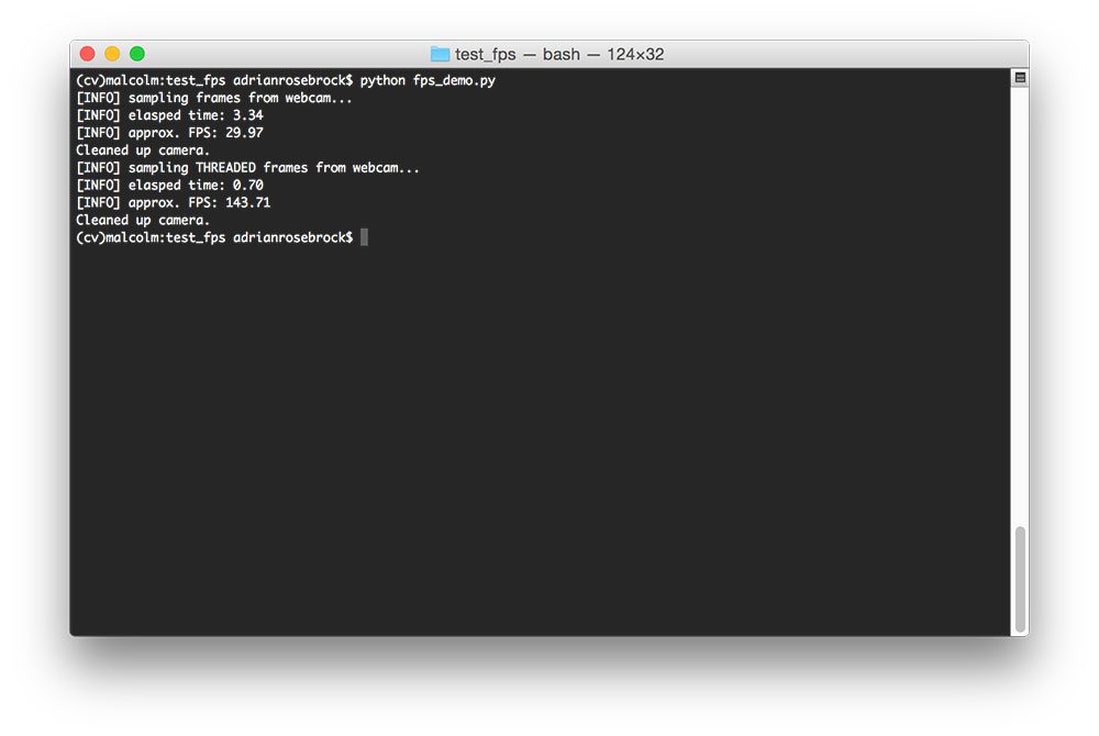
All that said, let’s give our OpenCV panorama stitcher a try. Open up a terminal and issue the following command:

$ python stitch.py --first images/bryce_left_01.png \
	--second images/bryce_right_01.png
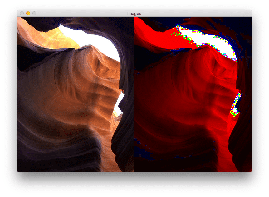
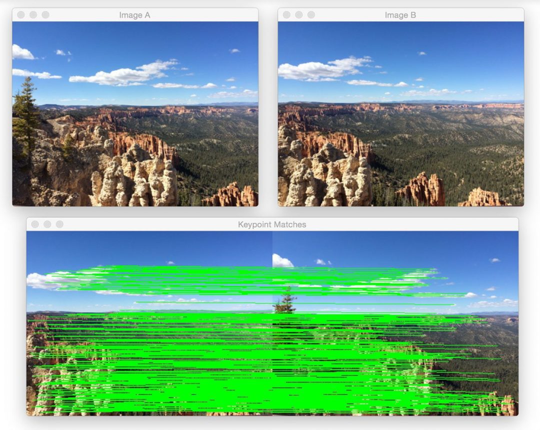
Figure 1: (Top) The two input images from Bryce canyon (in left-to-right order). (Bottom) The matched keypoint correspondences between the two images.

Figure 1: (Top) The two input images from Bryce canyon (in left-to-right order). (Bottom) The matched keypoint correspondences between the two images.

At the top of this figure, we can see two input images (resized to fit on my screen, the raw .jpg files are a much higher resolution). And on the bottom, we can see the matched keypoints between the two images.

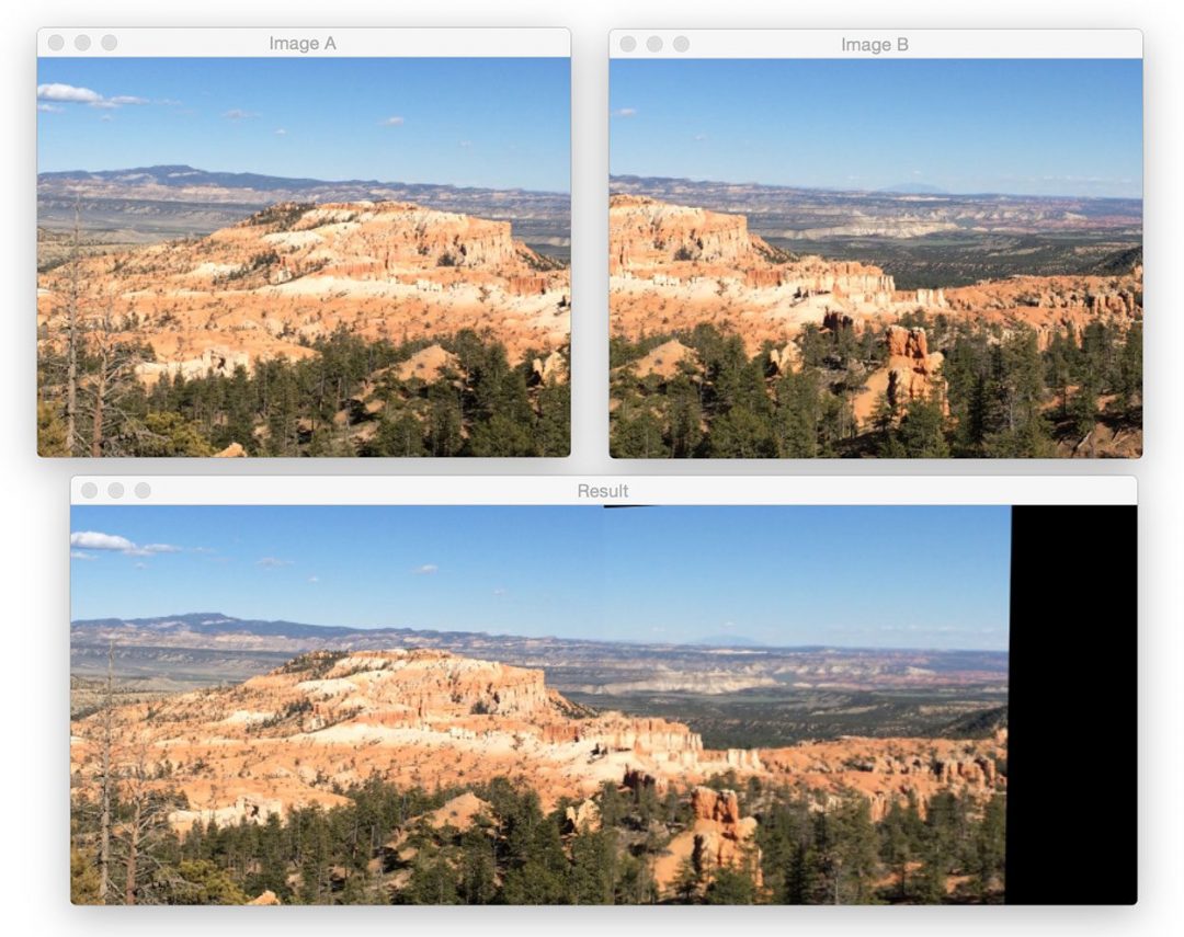
Using these matched keypoints, we can apply a perspective transform and obtain the final panorama:

Figure 2: Constructing a panorama from our two input images.

Figure 2: Constructing a panorama from our two input images.

As we can see, the two images have been successfully stitched together!

Note: On many of these example images, you’ll often see a visible “seam” running through the center of the stitched images. This is because I shot many of photos using either my iPhone or a digital camera with autofocus turned on, thus the focus is slightly different between each shot. Image stitching and panorama construction work best when you use the same focus for every photo. I never intended to use these vacation photos for image stitching, otherwise I would have taken care to adjust the camera sensors. In either case, just keep in mind the seam is due to varying sensor properties at the time I took the photo and was not intentional.

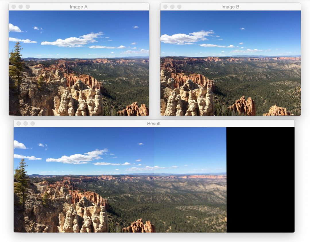
Let’s give another set of images a try:

$ python stitch.py --first images/bryce_left_02.png \
	--second images/bryce_right_02.png

Figure 3: Another successful application of image stitching with OpenCV.

Figure 3: Another successful application of image stitching with OpenCV.

Again, our

Stitcher
  class was able to construct a panorama from the two input images.

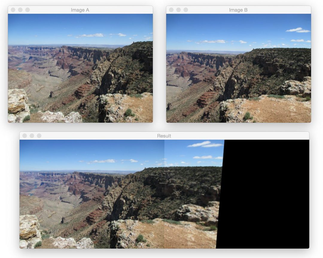
Now, let’s move on to the Grand Canyon:

$ python stitch.py --first images/grand_canyon_left_01.png \
	--second images/grand_canyon_right_01.png

Figure 4: Applying image stitching and panorama construction using OpenCV.

Figure 4: Applying image stitching and panorama construction using OpenCV.

In the above input images we can see heavy overlap between the two input images. The main addition to the panorama is towards the right side of the stitched images where we can see more of the “ledge” is added to the output.

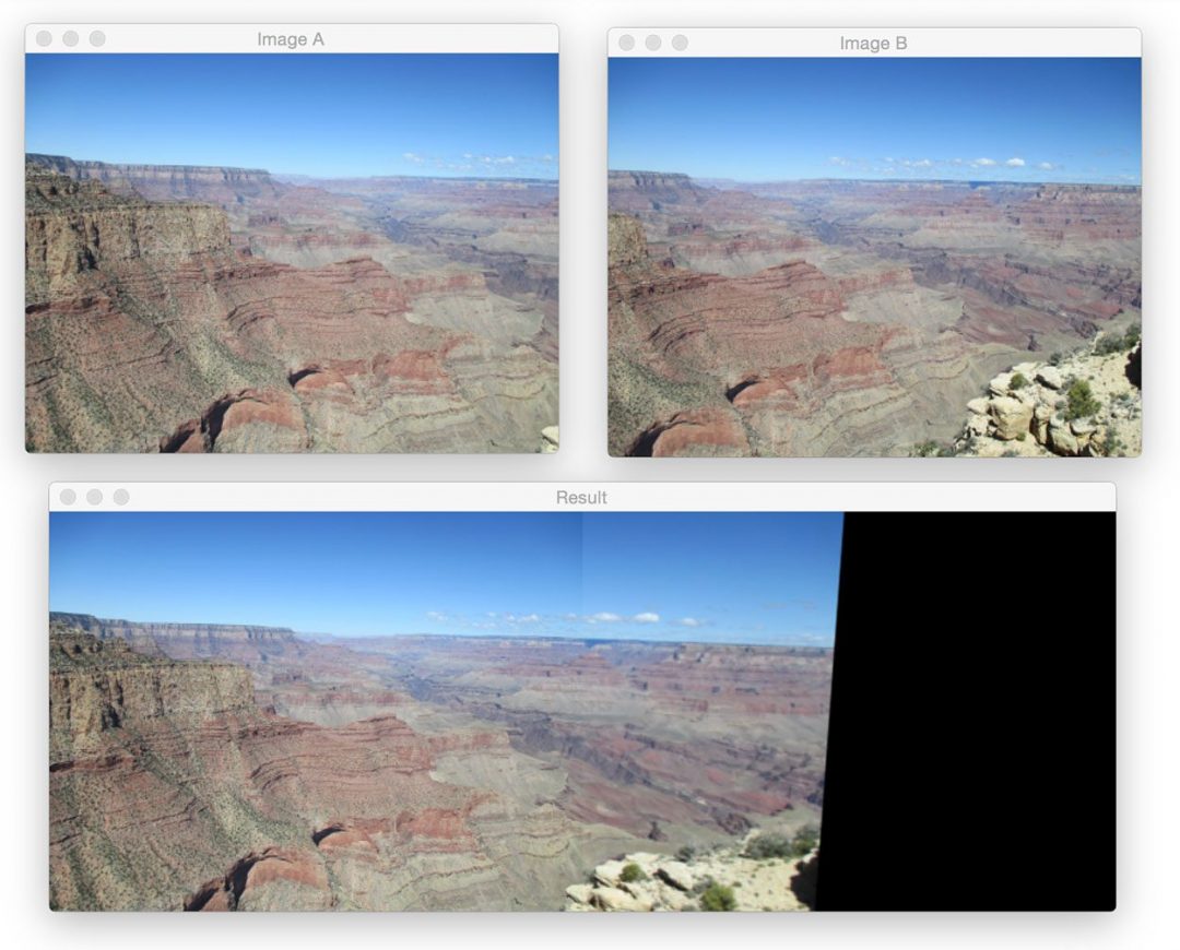
Here’s another example from the Grand Canyon:

$ python stitch.py --first images/grand_canyon_left_02.png \
	--second images/grand_canyon_right_02.png

Figure 5: Using image stitching to build a panorama using OpenCV and Python.

Figure 5: Using image stitching to build a panorama using OpenCV and Python.

From this example, we can see that more of the huge expanse of the Grand Canyon has been added to the panorama.

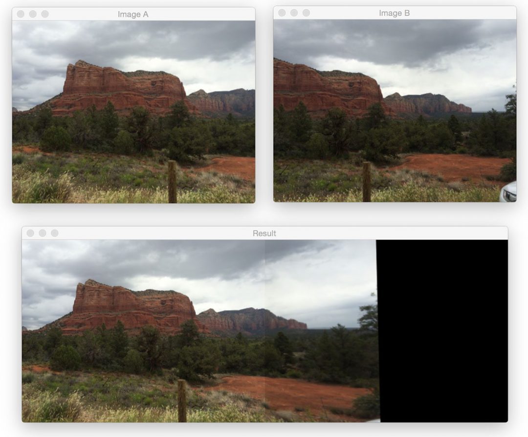
Finally, let’s wrap up this blog post with an example image stitching from Sedona, AZ:

$ python stitch.py --first images/sedona_left_01.png \
	--second images/sedona_right_01.png

Figure 6: One final example of applying image stitching.

Figure 6: One final example of applying image stitching.

Personally, I find the red rock country of Sedona to be one of the most beautiful areas I’ve ever visited. If you ever have a chance, definitely stop by — you won’t be disappointed.

So there you have it, image stitching and panorama construction using Python and OpenCV!

Summary

In this blog post we learned how to perform image stitching and panorama construction using OpenCV. Source code was provided for image stitching for both OpenCV 2.4 and OpenCV 3.

Our image stitching algorithm requires four steps: (1) detecting keypoints and extracting local invariant descriptors; (2) matching descriptors between images; (3) applying RANSAC to estimate the homography matrix; and (4) applying a warping transformation using the homography matrix.

While simple, this algorithm works well in practice when constructing panoramas for two images. In a future blog post, we’ll review how to construct panoramas and perform image stitching for more than two images.

Anyway, I hope you enjoyed this post! Be sure to use the form below to download the source code and give it a try.

Downloads:

If you would like to download the code and images used in this post, please enter your email address in the form below. Not only will you get a .zip of the code, I’ll also send you a FREE 11-page Resource Guide on Computer Vision and Image Search Engines, including exclusive techniques that I don’t post on this blog! Sound good? If so, enter your email address and I’ll send you the code immediately!

The post OpenCV panorama stitching appeared first on PyImageSearch.

Viewing all 432 articles
Browse latest View live