![]()
Is the Rectified Adam (RAdam) optimizer actually better than the standard Adam optimizer? According to my 24 experiments, the answer is no, typically not (but there are cases where you do want to use it instead of Adam).
In Liu et al.’s 2018 paper, On the Variance of the Adaptive Learning Rate and Beyond, the authors claim that Rectified Adam can obtain:
- Better accuracy (or at least identical accuracy when compared to Adam)
- And in fewer epochs than standard Adam
The authors tested their hypothesis on three different datasets, including one NLP dataset and two computer vision datasets (ImageNet and CIFAR-10).
In each case Rectified Adam outperformed standard Adam…but failed to outperform standard Stochastic Gradient Descent (SGD)!
The Rectified Adam optimizer has some strong theoretical justifications — but as a deep learning practitioner, you need more than just theory — you need to see empirical results applied to a variety of datasets.
And perhaps more importantly, you need to obtain a mastery level experience operating/driving the optimizer (or a small subset of optimizers) as well.
Today is part two in our two-part series on the Rectified Adam optimizer:
- Rectified Adam (RAdam) optimizer with Keras (last week’s post)
- Is Rectified Adam actually *better* than Adam (today’s tutorial)
If you haven’t yet, go ahead and read part one to ensure you have a good understanding of how the Rectified Adam optimizer works.
From there, read today’s post to help you understand how to design, code, and run experiments used to compare deep learning optimizers.
To learn how to compare Rectified Adam to standard Adam, just keep reading!
Is Rectified Adam actually *better* than Adam?
In the first part of this tutorial, we’ll briefly discuss the Rectified Adam optimizer, including how it works and why it’s interesting to us as deep learning practitioners.
From there, I’ll guide you in designing and planning our set of experiments to compare Rectified Adam to Adam — you can use this section to learn how you design your own deep learning experiments as well.
We’ll then review the project structure for this post, including implementing our training and evaluation scripts by hand.
Finally, we’ll run our experiments, collect results, and ultimately decide is Rectified Adam actually better than Adam?
What is the Rectified Adam optimizer?
![]()
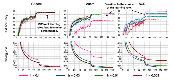
Figure 1: The Rectified Adam (RAdam) deep learning optimizer. Is it better than the standard Adam optimizer? (image source: Figure 6 from Liu et al.)
The Rectified Adam optimizer was proposed by Liu et al. in their 2019 paper, On the Variance of the Adaptive Learning Rate and Beyond. In their paper they discussed how their update to the Adam optimizer, called Rectified Adam, can:
- Obtain a higher accuracy/more generalizable deep neural network.
- Complete training in fewer epochs.
Their work had some strong theoretical justifications as well. They found that adaptive learning rate optimizers (such as Adam) both:
- Struggle to generalize during the first few batch updates
- Had very high variance
Liu et al. studied the problem in detail and found that the issue could be rectified (hence the name, Rectified Adam) by:
- Applying warm up with a low initial earning rate.
- Simply turning off the momentum term for the first few sets of input training batches.
The authors evaluated their experiments on one NLP dataset and two image classification datasets and found that their Rectified Adam implementation outperformed standard Adam (but neither optimizer outperformed standard SGD).
We’ll be continuing Liu et al.’s experiments today and comparing Rectified Adam to standard Adam in 24 separate experiments.
For more details on how the Rectified Adam optimizer works, be sure to review my previous blog post.
Planning our experiments
![]()
Figure 2: We will plan our set of experiments to evaluate the performance of the Rectified Adam (RAdam) optimizer using Keras.
To compare Adam to Rectified Adam, we’ll be training three Convolutional Neural Networks (CNNs), including:
- ResNet
- GoogLeNet
- MiniVGGNet
The implementations of these CNNs came directly from my book, Deep Learning for Computer Vision with Python.
These networks will be trained on four datasets:
- MNIST
- Fashion MNIST
- CIFAR-10
- CIFAR-100
For each combination of dataset and CNN architecture, we’ll apply two optimizers:
- Adam
- Rectified Adam
Taking all possible combinations, we end up with 3 x 4 x 2 = 24 separate training experiments.
We’ll run each of these experiments individually, collect, the results, and then interpret them to determine which optimizer is indeed better.
Whenever you plan your own experiments make sure you take the time to write out the list of model architectures, optimizers, and datasets you intend on applying them to. Additionally, you may want to list the hyperparameters you believe are important and are worth tuning (i.e., learning rate, L2 weight decay strength, etc.).
Considering the 24 experiments we plan to conduct, it makes the most sense to automate the data collection phase. From there, we will be able to work on other tasks while the computation is underway (often requiring days of compute time). Upon completion of the data collection for our 24 experiments, we will then be able to sit down and analyze the plots and classification reports in order to evaluate RAdam on our CNNs, datasets, and optimizers.
How to design your own deep learning experiments
![]()
Figure 3: Designing your own deep learning experiments, requires thought and planning. Consider your typical deep learning workflow and design your initial set of experiments such that a thorough preliminary investigation can be conducted using automation. Planning for automated evaluation now will save you time (and money) down the line.
Typically, my experiment design workflow goes something like this:
- Select 2-3 model architectures that I believe would work well on a particular dataset (i.e., ResNet, VGGNet, etc.).
- Decide if I want to train from scratch or perform transfer learning.
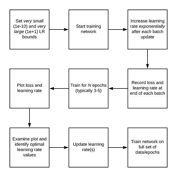
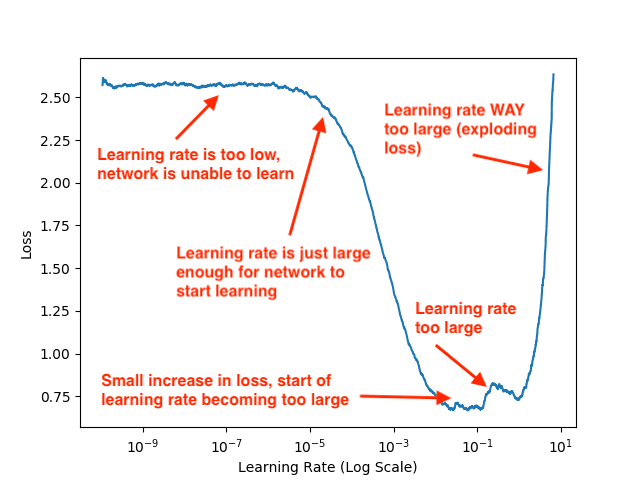
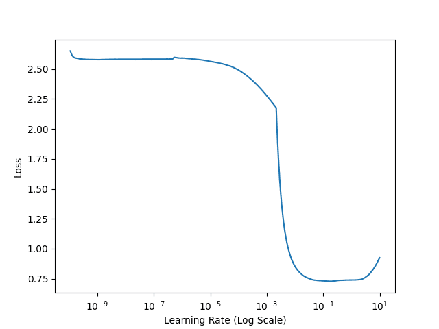
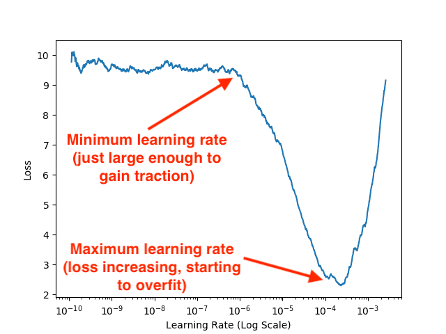
- Use my learning rate finder to find an acceptable initial learning rate for the SGD optimizer.
- Train the model on my dataset using SGD and Keras’ standard decay schedule.
- Look at my results from training, select the architecture that performed best, and start tuning my hyperparameters, including model capacity, regularization strength, revisiting the initial learning rate, applying Cyclical Learning Rates, and potentially exploring other optimizers.
You’ll notice that I tend to use SGD in my initial experiments instead of Adam, RMSprop, etc.
Why is that?
To answer that question you’ll need to read the “You need to obtain mastery level experience operating these three optimizers” section below.
Note: For more of my suggestions, tips, and best practices when designing and running your own experiments, be sure to refer to my book, Deep Learning for Computer Vision with Python.
However, in the context of this tutorial, we’re attempting to compare our results to the work of Liu et al.
We, therefore, need to fix the model architectures, training from scratch, learning rate, and optimizers — our experiment design now becomes:
- Train ResNet, GoogLeNet, and MiniVGGNet on MNIST, Fashion MNIST, CIFAR-10, and CIFAR-100, respectively.
- Train all networks from scratch.
- Use the initial, default learning rates for Adam/Rectified Adam (1e-3).
- Utilize the Adam and Rectified Adam optimizers for training.
- Since these are one-off experiments we’ll not be performing an exhaustive dive on tuning hyperparameters (you can refer to Deep Learning for Computer Vision with Python if you would like details on how to tune your hyperparameters).
At this point we’ve motivated and planned our set of experiments — now let’s learn how to implement our training and evaluation scripts.
Project structure
Go ahead and grab the “Downloads” and then inspect the project directory with the
tree
command:
$ tree --dirsfirst --filelimit 10
.
├── output [48 entries]
├── plots [12 entries]
├── pyimagesearch
│ ├── __init__.py
│ ├── minigooglenet.py
│ ├── minivggnet.py
│ └── resnet.py
├── combinations.py
├── experiments.sh
├── plot.py
└── train.py
3 directories, 68 files
Our project consists of two output directories:
output/
: Holds our classification report .txt
files organized by experiment. Additionally, there is one .pickle
file per experiment containing the serialized training history data (for plotting purposes).plots/
: For each CNN/dataset combination, a stacked accuracy/loss curve plot is output so that we can conveniently compare the Adam and RAdam optimizers.
The
pyimagesearch
module contains three Convolutional Neural Networks (CNNs) architectures constructed with Keras. These CNN implementations come directly from
Deep Learning for Computer Vision with Python.
We will review three Python scripts in today’s tutorial:
train.py
: Our training script accepts a CNN architecture, dataset, and optimizer via command line argument and begins fitting a model accordingly. This script will be invoked automatically for each of our 24 experiments via the experiments.sh
bash script. Our training script produces two types of output files:
.txt
: A classification report printout in scikit-learn’s standard format..pickle
: Serialized training history so that it can later be recalled for plotting purposes.
combinations.py
: This script computes all the experiment combinations for which we will train models and collect data. The result of executing this script is a bash/shell script named experiments.sh
.plot.py
: Plots accuracy/loss curves for Adam/RAdam using matplotlib directly from the output/*.pickle
files.
Implementing the training script
Our training script will be responsible for accepting:
- A given model architecture
- A dataset
- An optimizer
And from there, the script will handle training the specified model, on the supplied dataset, using the specified optimizer.
We’ll use this script to run each of our 24 experiments.
Let’s go ahead and implement the
train.py
script now:
# import the necessary packages
from pyimagesearch.minigooglenet import MiniGoogLeNet
from pyimagesearch.minivggnet import MiniVGGNet
from pyimagesearch.resnet import ResNet
from sklearn.preprocessing import LabelBinarizer
from sklearn.metrics import classification_report
from keras.preprocessing.image import ImageDataGenerator
from keras.optimizers import Adam
from keras_radam import RAdam
from keras.datasets import fashion_mnist
from keras.datasets import cifar100
from keras.datasets import cifar10
from keras.datasets import mnist
import numpy as np
import argparse
import pickle
import cv2
Imports include our three CNN architectures, four datasets, and two optimizers (
Adam
and
RAdam
).
Let’s parse command line arguments:
# construct the argument parser and parse the arguments
ap = argparse.ArgumentParser()
ap.add_argument("-i", "--history", required=True,
help="path to output training history file")
ap.add_argument("-r", "--report", required=True,
help="path to output classification report file")
ap.add_argument("-d", "--dataset", type=str, default="mnist",
choices=["mnist", "fashion_mnist", "cifar10", "cifar100"],
help="dataset name")
ap.add_argument("-m", "--model", type=str, default="resnet",
choices=["resnet", "googlenet", "minivggnet"],
help="type of model architecture")
ap.add_argument("-o", "--optimizer", type=str, default="adam",
choices=["adam", "radam"],
help="type of optmizer")
args = vars(ap.parse_args())Our command line arguments include:
--history
: The path to the output training history .pickle
file.--report
: The path to the output classification report .txt
file.--dataset
: The dataset to train our model on can be any of the choices
listed on Line 26.--model
: The deep learning model architecture must be one of the choices
on Line 29.--optimizer
: Our adam
or radam
deep learning optimization method.
Upon providing the command line arguments via the terminal, our training script dynamically sets up and launches the experiment. Output files are named according to the parameters of the experiment.
From here we’ll set two constants and initialize the default number of channels for the dataset:
# initialize the batch size and number of epochs to train
BATCH_SIZE = 128
NUM_EPOCHS = 60
# initialize the number of channels in the dataset
numChans = 1
If our
--dataset
is MNIST or Fashion MNIST, we’ll load the dataset in the following manner:
# check if we are using either the MNIST or Fashion MNIST dataset
if args["dataset"] in ("mnist", "fashion_mnist"):
# check if we are using MNIST
if args["dataset"] == "mnist":
# initialize the label names for the MNIST dataset
labelNames = [str(i) for i in range(0, 10)]
# load the MNIST dataset
print("[INFO] loading MNIST dataset...")
((trainX, trainY), (testX, testY)) = mnist.load_data()
# otherwise, are are using Fashion MNIST
else:
# initialize the label names for the Fashion MNIST dataset
labelNames = ["top", "trouser", "pullover", "dress", "coat",
"sandal", "shirt", "sneaker", "bag", "ankle boot"]
# load the Fashion MNIST dataset
print("[INFO] loading Fashion MNIST dataset...")
((trainX, trainY), (testX, testY)) = fashion_mnist.load_data()
# MNIST dataset images are 28x28 but the networks we will be
# training expect 32x32 images
trainX = np.array([cv2.resize(x, (32, 32)) for x in trainX])
testX = np.array([cv2.resize(x, (32, 32)) for x in testX])
# reshape the data matrices to include a channel dimension which
# is required for training)
trainX = trainX.reshape((trainX.shape[0], 32, 32, 1))
testX = testX.reshape((testX.shape[0], 32, 32, 1))Keep in mind that MNIST images are 28×28 but we need 32×32 images for our architectures. Thus, Lines 66 and 67
resize
all images in the dataset.
Lines 71 and 72 then add the batch dimension.
Otherwise, we have a CIFAR variant
--dataset
to load:
# otherwise, we must be using a variant of CIFAR
else:
# update the number of channels in the images
numChans = 3
# check if we are using CIFAR-10
if args["dataset"] == "cifar10":
# initialize the label names for the CIFAR-10 dataset
labelNames = ["airplane", "automobile", "bird", "cat",
"deer", "dog", "frog", "horse", "ship", "truck"]
# load the CIFAR-10 dataset
print("[INFO] loading CIFAR-10 dataset...")
((trainX, trainY), (testX, testY)) = cifar10.load_data()
# otherwise, we are using CIFAR-100
else:
# initialize the label names for the CIFAR-100 dataset
labelNames = ["apple", "aquarium_fish", "baby", "bear",
"beaver", "bed", "bee", "beetle", "bicycle", "bottle",
"bowl", "boy", "bridge", "bus", "butterfly", "camel",
"can", "castle", "caterpillar", "cattle", "chair",
"chimpanzee", "clock", "cloud", "cockroach", "couch",
"crab", "crocodile", "cup", "dinosaur", "dolphin",
"elephant", "flatfish", "forest", "fox", "girl",
"hamster", "house", "kangaroo", "keyboard", "lamp",
"lawn_mower", "leopard", "lion", "lizard", "lobster",
"man", "maple_tree", "motorcycle", "mountain", "mouse",
"mushroom", "oak_tree", "orange", "orchid", "otter",
"palm_tree", "pear", "pickup_truck", "pine_tree", "plain",
"plate", "poppy", "porcupine", "possum", "rabbit",
"raccoon", "ray", "road", "rocket", "rose", "sea", "seal",
"shark", "shrew", "skunk", "skyscraper", "snail", "snake",
"spider", "squirrel", "streetcar", "sunflower",
"sweet_pepper", "table", "tank", "telephone", "television",
"tiger", "tractor", "train", "trout", "tulip", "turtle",
"wardrobe", "whale", "willow_tree", "wolf", "woman", "worm"]
# load the CIFAR-100 dataset
print("[INFO] loading CIFAR-100 dataset...")
((trainX, trainY), (testX, testY)) = cifar100.load_data()CIFAR datasets contain 3-channel color images (Line 77). These datasets are already comprised of 32×32 images (no resizing is necessary).
From here, we’ll scale our data and determine the total number of classes:
# scale the data to the range [0, 1]
trainX = trainX.astype("float32") / 255.0
testX = testX.astype("float32") / 255.0
# determine the total number of unique classes in the dataset
numClasses = len(np.unique(trainY))
print("[INFO] {} classes in dataset".format(numClasses))Followed by initializing this experiment’s deep learning optimizer:
# check if we are using Adam
if args["optimizer"] == "adam":
# initialize the Adam optimizer
print("[INFO] using Adam optimizer")
opt = Adam(lr=1e-3)
# otherwise, we are using Rectified Adam
else:
# initialize the Rectified Adam optimizer
print("[INFO] using Rectified Adam optimizer")
opt = RAdam(total_steps=5000, warmup_proportion=0.1, min_lr=1e-5)Either
Adam
or
RAdam
is initialized according to the
--optimizer
command line argument switch.
Our
model
is then built depending upon the
--model
command line argument:
# check if we are using the ResNet architecture
if args["model"] == "resnet":
# utilize the ResNet architecture
print("[INFO] initializing ResNet...")
model = ResNet.build(32, 32, numChans, numClasses, (9, 9, 9),
(64, 64, 128, 256), reg=0.0005)
# check if we are using Tiny GoogLeNet
elif args["model"] == "googlenet":
# utilize the MiniGoogLeNet architecture
print("[INFO] initializing MiniGoogLeNet...")
model = MiniGoogLeNet.build(width=32, height=32, depth=numChans,
classes=numClasses)
# otherwise, we must be using MiniVGGNet
else:
# utilize the MiniVGGNet architecture
print("[INFO] initializing MiniVGGNet...")
model = MiniVGGNet.build(width=32, height=32, depth=numChans,
classes=numClasses)Once either ResNet, GoogLeNet, or MiniVGGNet is built, we’ll binarize our labels and construct our data augmentation object:
# convert the labels from integers to vectors
lb = LabelBinarizer()
trainY = lb.fit_transform(trainY)
testY = lb.transform(testY)
# construct the image generator for data augmentation
aug = ImageDataGenerator(rotation_range=18, zoom_range=0.15,
width_shift_range=0.2, height_shift_range=0.2, shear_range=0.15,
horizontal_flip=True, fill_mode="nearest")
Followed by compiling our model and training the network:
# compile the model and train the network
print("[INFO] training network...")
model.compile(loss="categorical_crossentropy", optimizer=opt,
metrics=["accuracy"])
H = model.fit_generator(
aug.flow(trainX, trainY, batch_size=BATCH_SIZE),
validation_data=(testX, testY),
steps_per_epoch=trainX.shape[0] // BATCH_SIZE,
epochs=NUM_EPOCHS,
verbose=1)We then evaluate the trained model and dump training history to disk:
# evaluate the network
print("[INFO] evaluating network...")
predictions = model.predict(testX, batch_size=BATCH_SIZE)
report = classification_report(testY.argmax(axis=1),
predictions.argmax(axis=1), target_names=labelNames)
# serialize the training history to disk
print("[INFO] serializing training history...")
f = open(args["history"], "wb")
f.write(pickle.dumps(H.history))
f.close()
# save the classification report to disk
print("[INFO] saving classification report...")
f = open(args["report"], "w")
f.write(report)
f.close()Each experiment will contain a classification report
.txt
file along with a serialized training history
.pickle
file.
The classification reports will be inspected manually whereas the training history files will later be opened by operations inside
plot.py
, the training history parsed, and finally plotted.
As you’ve learned, creating a training script that dynamically sets up an experiment is quite straightforward.
Creating our experiment combinations
At this point, we have our training script which can accept a (1) model architecture, (2) dataset, and (3) optimizer, followed by fitting a model using the respective combination.
That being said, are we going to manually run each and every individual command?
No, not only is that a tedious task, it’s also prone to human error.
Instead, let’s create a Python script to generate a shell script containing the train.py
command for each experiment we want to run.
Open up the
combinations.py
file and insert the following code:
# import the necessary packages
import argparse
import os
# construct the argument parser and parse the arguments
ap = argparse.ArgumentParser()
ap.add_argument("-o", "--output", required=True,
help="path to output output directory")
ap.add_argument("-s", "--script", required=True,
help="path to output shell script")
args = vars(ap.parse_args())Our script requires two command line arguments:
--output
: The path to the output directory where the training files will be stored.--script
: The path to the output shell script which will contain all of our training script commands with command line argument combinations.
Let’s go ahead and open a new file for writing:
# open the output shell script for writing, then write the header
f = open(args["script"], "w")
f.write("#!/bin/sh\n\n")
# initialize the list of datasets, models, and optimizers
datasets = ["mnist", "fashion_mnist", "cifar10", "cifar100"]
models = ["resnet", "googlenet", "minivggnet"]
optimizers = ["adam", "radam"]Line 14 opens a shell script file writing. Subsequently, Line 15 writes the “shebang” to indicate that this shell script is executable.
Lines 18-20 then list our
datasets
,
models
, and
optimizers
.
We will form all possible combinations of experiments from these lists in a nested loop:
# loop over all combinations of datasets, models, and optimizers
for dataset in datasets:
for model in models:
for opt in optimizers:
# build the path to the output training log file
histFilename = "{}_{}_{}.pickle".format(model, opt, dataset)
historyPath = os.path.sep.join([args["output"],
histFilename])
# build the path to the output report log file
reportFilename = "{}_{}_{}.txt".format(model, opt, dataset)
reportPath = os.path.sep.join([args["output"],
reportFilename])
# construct the command that will be executed to launch
# the experiment
cmd = ("python train.py --history {} --report {} "
"--dataset {} --model {} --optimizer {}").format(
historyPath, reportPath, dataset, model, opt)
# write the command to disk
f.write("{}\n".format(cmd))
# close the shell script file
f.close()Inside the loop, we:
- Construct our history file path (Lines 27-29).
- Assemble our report file path (Lines 32-34).
- Concatenate each command per the current loop iteration’s combination and write it to the shell file (Lines 38-43).
Finally, we close the shell script file.
Note: I am making the assumption that you are using a Unix machine to run these experiments. If you’re using Windows you should either (1) update this script to generate a batch file instead, or (2) manually execute the train.py
command for each respective experiment. Note that I do not support Windows on the PyImageSearch blog so you will be on your own to implement it based on this script.
Generating the experiment shell script
Go ahead and use the “Downloads” section of this tutorial to download the source code to the guide.
From there, open up a terminal and execute the
combinations.py
script:
$ python combinations.py --output output --script experiments.sh
After the script has executed you should have a file named
experiments.sh
in your working directory — this file contains the 24 separate experiments we’ll be running to compare Adam to Rectified Adam.
Go ahead and investigate
experiments.sh
now:
#!/bin/sh
python train.py --history output/resnet_adam_mnist.pickle --report output/resnet_adam_mnist.txt --dataset mnist --model resnet --optimizer adam
python train.py --history output/resnet_radam_mnist.pickle --report output/resnet_radam_mnist.txt --dataset mnist --model resnet --optimizer radam
python train.py --history output/googlenet_adam_mnist.pickle --report output/googlenet_adam_mnist.txt --dataset mnist --model googlenet --optimizer adam
python train.py --history output/googlenet_radam_mnist.pickle --report output/googlenet_radam_mnist.txt --dataset mnist --model googlenet --optimizer radam
python train.py --history output/minivggnet_adam_mnist.pickle --report output/minivggnet_adam_mnist.txt --dataset mnist --model minivggnet --optimizer adam
python train.py --history output/minivggnet_radam_mnist.pickle --report output/minivggnet_radam_mnist.txt --dataset mnist --model minivggnet --optimizer radam
python train.py --history output/resnet_adam_fashion_mnist.pickle --report output/resnet_adam_fashion_mnist.txt --dataset fashion_mnist --model resnet --optimizer adam
python train.py --history output/resnet_radam_fashion_mnist.pickle --report output/resnet_radam_fashion_mnist.txt --dataset fashion_mnist --model resnet --optimizer radam
python train.py --history output/googlenet_adam_fashion_mnist.pickle --report output/googlenet_adam_fashion_mnist.txt --dataset fashion_mnist --model googlenet --optimizer adam
python train.py --history output/googlenet_radam_fashion_mnist.pickle --report output/googlenet_radam_fashion_mnist.txt --dataset fashion_mnist --model googlenet --optimizer radam
python train.py --history output/minivggnet_adam_fashion_mnist.pickle --report output/minivggnet_adam_fashion_mnist.txt --dataset fashion_mnist --model minivggnet --optimizer adam
python train.py --history output/minivggnet_radam_fashion_mnist.pickle --report output/minivggnet_radam_fashion_mnist.txt --dataset fashion_mnist --model minivggnet --optimizer radam
python train.py --history output/resnet_adam_cifar10.pickle --report output/resnet_adam_cifar10.txt --dataset cifar10 --model resnet --optimizer adam
python train.py --history output/resnet_radam_cifar10.pickle --report output/resnet_radam_cifar10.txt --dataset cifar10 --model resnet --optimizer radam
python train.py --history output/googlenet_adam_cifar10.pickle --report output/googlenet_adam_cifar10.txt --dataset cifar10 --model googlenet --optimizer adam
python train.py --history output/googlenet_radam_cifar10.pickle --report output/googlenet_radam_cifar10.txt --dataset cifar10 --model googlenet --optimizer radam
python train.py --history output/minivggnet_adam_cifar10.pickle --report output/minivggnet_adam_cifar10.txt --dataset cifar10 --model minivggnet --optimizer adam
python train.py --history output/minivggnet_radam_cifar10.pickle --report output/minivggnet_radam_cifar10.txt --dataset cifar10 --model minivggnet --optimizer radam
python train.py --history output/resnet_adam_cifar100.pickle --report output/resnet_adam_cifar100.txt --dataset cifar100 --model resnet --optimizer adam
python train.py --history output/resnet_radam_cifar100.pickle --report output/resnet_radam_cifar100.txt --dataset cifar100 --model resnet --optimizer radam
python train.py --history output/googlenet_adam_cifar100.pickle --report output/googlenet_adam_cifar100.txt --dataset cifar100 --model googlenet --optimizer adam
python train.py --history output/googlenet_radam_cifar100.pickle --report output/googlenet_radam_cifar100.txt --dataset cifar100 --model googlenet --optimizer radam
python train.py --history output/minivggnet_adam_cifar100.pickle --report output/minivggnet_adam_cifar100.txt --dataset cifar100 --model minivggnet --optimizer adam
python train.py --history output/minivggnet_radam_cifar100.pickle --report output/minivggnet_radam_cifar100.txt --dataset cifar100 --model minivggnet --optimizer radam
Note: Be sure to use the horizontal scroll bar to inspect the entire contents of the experiments.sh
script. I intentionally did not break up lines or automatically wrap them for better display. You can also refer to Figure 4 below — I suggest clicking the image to enlarge + inspect it.
![]()
Figure 4: The output of our combinations.py file is a shell script listing the training script commands to run in succession. Click image to enlarge.
Notice how there is a
train.py
call for
each of the 24 possible combinations of model architecture, dataset, and optimizer. Furthermore, the “shebang” on
Line 1 indicates that this shell script is executable.
Running our experiments
The next step is to actually perform each of these experiments.
I executed the shell script on an Amazon EC2 instance with an NVIDIA K80 GPU. It took approximately 48 hours to run all the experiments.
To launch the experiments for yourself, just run the following command:
$ ./experiments.sh
After the script has finished running, your
output/
directory should be filled with
.pickle
and
.txt
files:
$ ls -l output/
googlenet_adam_cifar10.pickle
googlenet_adam_cifar10.txt
googlenet_adam_cifar100.pickle
googlenet_adam_cifar100.txt
...
resnet_radam_fashion_mnist.pickle
resnet_radam_fashion_mnist.txt
resnet_radam_mnist.pickle
resnet_radam_mnist.txt
The
.txt
files contain the output of scikit-learn’s
classification_report
, a human-readable output that tells us how well our model performed.
The
.pickle
files contain the training history for the model. We’ll use this
.pickle
file to plot both Adam and Rectified Adam’s performance in the next section.
Implementing our Adam vs. Rectified Adam plotting script
Our final Python script,
plot.py
, will be used to plot the performance of Adam vs. Rectified Adam, giving us a nice, clear visualization of a given model architecture trained on a specific dataset.
The plot file opens each Adam/RAdam
.pickle
file pair and generates a corresponding plot.
Open up
plot.py
and insert the following code:
# import the necessary packages
import matplotlib.pyplot as plt
import numpy as np
import argparse
import pickle
import os
def plot_history(adamHist, rAdamHist, accTitle, lossTitle):
# determine the total number of epochs used for training, then
# initialize the figure
N = np.arange(0, len(adamHist["loss"]))
plt.style.use("ggplot")
(fig, axs) = plt.subplots(2, 1, figsize=(7, 9))
# plot the accuracy for Adam vs. Rectified Adam
axs[0].plot(N, adamHist["acc"], label="adam_train_acc")
axs[0].plot(N, adamHist["val_acc"], label="adam_val_acc")
axs[0].plot(N, rAdamHist["acc"], label="radam_train_acc")
axs[0].plot(N, rAdamHist["val_acc"], label="radam_val_acc")
axs[0].set_title(accTitle)
axs[0].set_xlabel("Epoch #")
axs[0].set_ylabel("Accuracy")
axs[0].legend(loc="lower right")
# plot the loss for Adam vs. Rectified Adam
axs[1].plot(N, adamHist["loss"], label="adam_train_loss")
axs[1].plot(N, adamHist["val_loss"], label="adam_val_loss")
axs[1].plot(N, rAdamHist["loss"], label="radam_train_loss")
axs[1].plot(N, rAdamHist["val_loss"], label="radam_val_loss")
axs[1].set_title(lossTitle)
axs[1].set_xlabel("Epoch #")
axs[1].set_ylabel("Loss")
axs[1].legend(loc="upper right")
# update the layout of the plot
plt.tight_layout()Lines 2-6 handle imports, namely the
matplotlib.pyplot
module.
The
plot_history
function is responsible for generating two stacked plots via the subplots feature:
- Training/validation accuracy curves (Lines 16-23).
- Training/validation loss curves (Lines 26-33).
Both Adam and Rectified Adam training history curves are generated from
adamHist
and
rAdamHist
data passed as parameters to the function.
Note: If you are using TensorFlow 2.0 (i.e., tf.keras
) to run this code , you’ll need to change all occurrences of acc
and val_acc
to accuracy
and val_accuracy
, respectively as TensorFlow 2.0 has made a breaking change to the accuracy name.
Let’s handle parsing command line arguments:
# construct the argument parser and parse the arguments
ap = argparse.ArgumentParser()
ap.add_argument("-i", "--input", required=True,
help="path to input directory of Keras training history files")
ap.add_argument("-p", "--plots", required=True,
help="path to output directory of training plots")
args = vars(ap.parse_args())
# initialize the list of datasets and models
datasets = ["mnist", "fashion_mnist", "cifar10", "cifar100"]
models = ["resnet", "googlenet", "minivggnet"]Our command line arguments consist of:
--input
: The path to the input directory of training history files to be parsed for plot generation.--plots
: Our output path where the plots will be stored.
Lines 47 and 48 list our
datasets
and
models
. We’ll loop over the combinations of datasets and models to generate our plots:
# loop over all combinations of datasets and models
for dataset in datasets:
for model in models:
# construct the path to the Adam output training history files
adamFilename = "{}_{}_{}.pickle".format(model, "adam",
dataset)
adamPath = os.path.sep.join([args["input"], adamFilename])
# construct the path to the Rectified Adam output training
# history files
rAdamFilename = "{}_{}_{}.pickle".format(model, "radam",
dataset)
rAdamPath = os.path.sep.join([args["input"], rAdamFilename])
# load the training history files for Adam and Rectified Adam,
# respectively
adamHist = pickle.loads(open(adamPath, "rb").read())
rAdamHist = pickle.loads(open(rAdamPath, "rb").read())
# plot the accuracy/loss for the current dataset, comparing
# Adam vs. Rectified Adam
accTitle = "Adam vs. RAdam for '{}' on '{}' (Accuracy)".format(
model, dataset)
lossTitle = "Adam vs. RAdam for '{}' on '{}' (Loss)".format(
model, dataset)
plot_history(adamHist, rAdamHist, accTitle, lossTitle)
# construct the path to the output plot
plotFilename = "{}_{}.png".format(model, dataset)
plotPath = os.path.sep.join([args["plots"], plotFilename])
# save the plot and clear it
plt.savefig(plotPath)
plt.clf()Inside our nested
datasets
/
models
loop, we:
- Construct Adam and Rectified Adam’s file paths (Lines 54-62).
- Load serialized training history (Lines 66 and 67).
- Generate the plots using our
plot_history
function (Lines 71-75).
- Export the figures to disk (Lines 78-83).
Plotting Adam vs. Rectified Adam
We are now ready to run the
plot.py
script.
Again, make sure you have used the “Downloads” section of this tutorial to download the source code.
From there, execute the following command:
$ python plot.py --input output --plots plots
You can then check the
plots/
directory and ensure it has been populated with the training history figures:
$ ls -l plots/
googlenet_cifar10.png
googlenet_cifar100.png
googlenet_fashion_mnist.png
googlenet_mnist.png
minivggnet_cifar10.png
minivggnet_cifar100.png
minivggnet_fashion_mnist.png
minivggnet_mnist.png
resnet_cifar10.png
resnet_cifar100.png
resnet_fashion_mnist.png
resnet_mnist.png
In the next section, we’ll review the results of our experiments.
Adam vs. Rectified Adam Experiments with MNIST
![]()
Figure 5: Montage of samples from the MNIST digit dataset.
Our first set of experiments will compare Adam vs. Rectified Adam on the MNIST dataset, a standard benchmark image classification dataset for handwritten digit recognition.
MNIST – MiniVGGNet
![]()
Figure 6: Which is better — Adam or RAdam optimizer using MiniVGGNet on the MNIST dataset?
Our first experiment compares Adam to Rectified Adam when training MiniVGGNet on the MNIST dataset.
Below is the output classification report for the Adam optimizer:
precision recall f1-score support
0 0.99 1.00 1.00 980
1 0.99 1.00 0.99 1135
2 0.98 0.96 0.97 1032
3 1.00 1.00 1.00 1010
4 0.99 1.00 0.99 982
5 0.97 0.98 0.98 892
6 0.98 0.98 0.98 958
7 0.99 0.99 0.99 1028
8 0.99 0.99 0.99 974
9 1.00 0.99 0.99 1009
micro avg 0.99 0.99 0.99 10000
macro avg 0.99 0.99 0.99 10000
weighted avg 0.99 0.99 0.99 10000As well as the classification report for the Rectified Adam optimizer:
precision recall f1-score support
0 0.99 1.00 0.99 980
1 1.00 0.99 1.00 1135
2 0.97 0.97 0.97 1032
3 0.99 0.99 0.99 1010
4 0.99 0.99 0.99 982
5 0.98 0.97 0.97 892
6 0.98 0.98 0.98 958
7 0.99 0.99 0.99 1028
8 0.99 0.99 0.99 974
9 0.99 0.99 0.99 1009
micro avg 0.99 0.99 0.99 10000
macro avg 0.99 0.99 0.99 10000
weighted avg 0.99 0.99 0.99 10000As you can see, we’re obtaining 99% accuracy for both experiments.
Looking at Figure 6 you can observe the warmup period associated with Rectified Adam:
Loss starts off very high and accuracy very low
After warmup is complete the Rectified Adam optimizer catches up with Adam
What’s interesting to note though is that Adam obtains lower loss compared to Rectified Adam — we’ll actually see that trend continue in the rest of the experiments we run (and I’ll explain why this happens as well).
MNIST – GoogLeNet
![]()
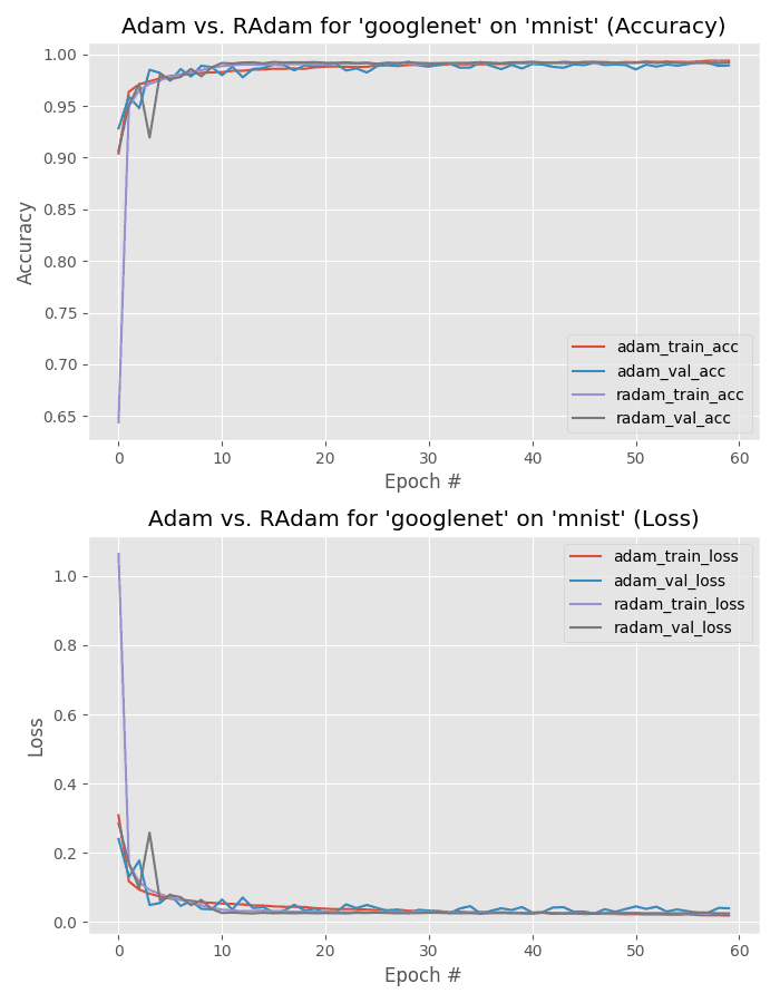
Figure 7: Which deep learning optimizer is actually better — Rectified Adam or Adam? This plot is from my experiment notebook while testing RAdam and Adam using GoogLeNet on the MNIST dataset.
This next experiment compares Adam to Rectified Adam for GoogLeNet trained on the MNIST dataset.
Below follows the output of the Adam optimizer:
precision recall f1-score support
0 1.00 1.00 1.00 980
1 1.00 0.99 1.00 1135
2 0.96 0.99 0.97 1032
3 0.99 1.00 0.99 1010
4 0.99 0.99 0.99 982
5 0.99 0.96 0.98 892
6 0.98 0.99 0.98 958
7 0.99 0.99 0.99 1028
8 1.00 1.00 1.00 974
9 1.00 0.98 0.99 1009
micro avg 0.99 0.99 0.99 10000
macro avg 0.99 0.99 0.99 10000
weighted avg 0.99 0.99 0.99 10000As well as the output for the Rectified Adam optimizer:
precision recall f1-score support
0 1.00 1.00 1.00 980
1 1.00 0.99 1.00 1135
2 0.98 0.98 0.98 1032
3 1.00 0.99 1.00 1010
4 1.00 0.99 1.00 982
5 0.97 0.99 0.98 892
6 0.99 0.98 0.99 958
7 0.99 1.00 0.99 1028
8 0.99 1.00 1.00 974
9 1.00 0.99 1.00 1009
micro avg 0.99 0.99 0.99 10000
macro avg 0.99 0.99 0.99 10000
weighted avg 0.99 0.99 0.99 10000Again, 99% accuracy is obtained for both optimizers.
This time both the training/validation plots are near identical for both accuracy and loss.
MNIST – ResNet
![]()
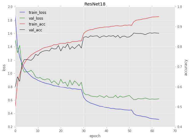
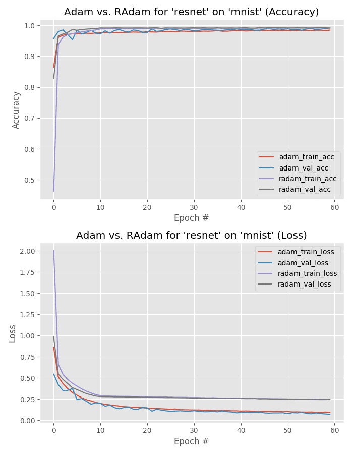
Figure 8: Training accuracy/loss plot for ResNet on the MNIST dataset using both the RAdam (Rectified Adam) and Adam deep learning optimizers with Keras.
Our final MNIST experiment compares training ResNet using both Adam and Rectified Adam.
Given that MNIST is not a very challenging dataset we obtain 99% accuracy for the Adam optimizer:
precision recall f1-score support
0 1.00 1.00 1.00 980
1 1.00 0.99 1.00 1135
2 0.98 0.98 0.98 1032
3 0.99 1.00 1.00 1010
4 0.99 1.00 0.99 982
5 0.99 0.98 0.98 892
6 0.98 0.99 0.99 958
7 0.99 1.00 0.99 1028
8 0.99 1.00 1.00 974
9 1.00 0.98 0.99 1009
micro avg 0.99 0.99 0.99 10000
macro avg 0.99 0.99 0.99 10000
weighted avg 0.99 0.99 0.99 10000As well as the Rectified Adam optimizer:
precision recall f1-score support
0 1.00 1.00 1.00 980
1 1.00 1.00 1.00 1135
2 0.97 0.98 0.98 1032
3 1.00 1.00 1.00 1010
4 0.99 1.00 1.00 982
5 0.99 0.97 0.98 892
6 0.99 0.98 0.99 958
7 0.99 1.00 0.99 1028
8 1.00 1.00 1.00 974
9 1.00 0.99 1.00 1009
micro avg 0.99 0.99 0.99 10000
macro avg 0.99 0.99 0.99 10000
weighted avg 0.99 0.99 0.99 10000But take a look at Figure 8 — note how Adam obtains much lower loss than Rectified Adam.
That’s not necessarily a bad thing as it may imply that Rectified Adam is obtaining a more generalizable model; however, performance on the testing set is identical so we would need to test on images outside MNIST (which is outside the scope of this blog post).
Adam vs. Rectified Adam Experiments with Fashion MNIST
![]()
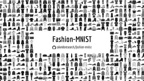
Figure 9: The Fashion MNIST dataset was created by e-commerce company, Zalando, as a drop-in replacement for MNIST Digits. It is a great dataset to practice/experiment with when using Keras for deep learning. (image source)
Our next set of experiments evaluate Adam vs. Rectified Adam on the Fashion MNIST dataset, a drop-in replacement for the standard MNIST dataset.
You can read more about Fashion MNIST here.
Fashion MNIST – MiniVGGNet
![]()
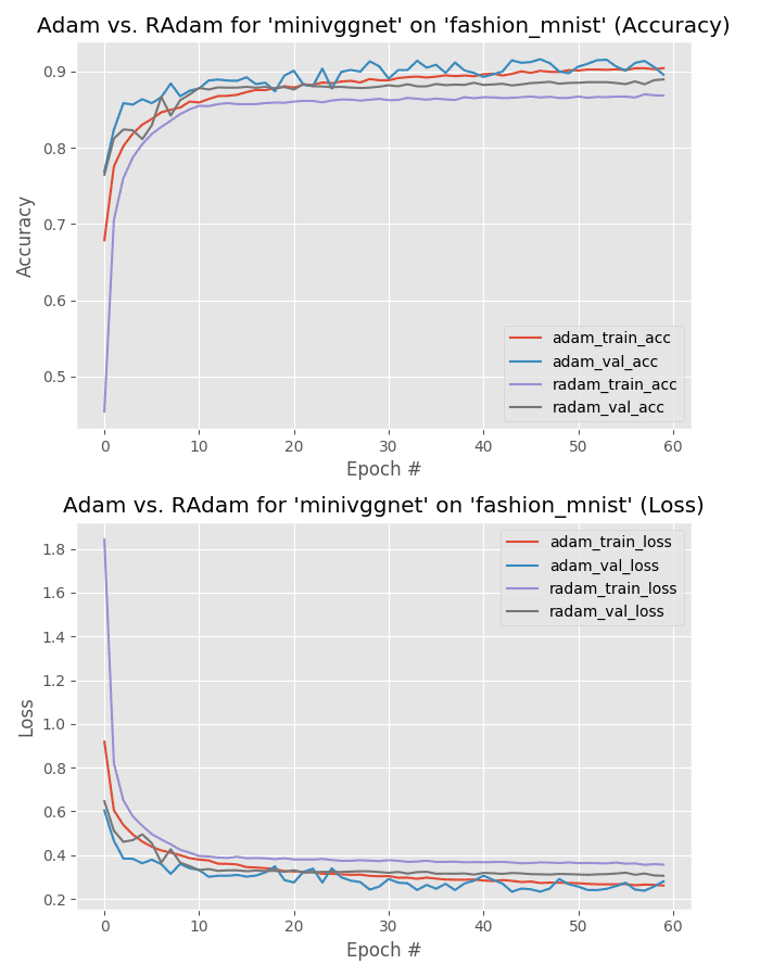
Figure 10: Testing optimizers with deep learning, including new ones such as RAdam, requires multiple experiments. Shown in this figure is the MiniVGGNet CNN trained on the Fashion MNIST dataset with both Adam and RAdam optimizers.
Our first experiment evaluates the MiniVGGNet architecture trained on the Fashion MNIST dataset.
Below you can find the output of training with the Adam optimizer:
precision recall f1-score support
top 0.95 0.71 0.81 1000
trouser 0.99 0.99 0.99 1000
pullover 0.94 0.76 0.84 1000
dress 0.96 0.80 0.87 1000
coat 0.84 0.90 0.87 1000
sandal 0.98 0.98 0.98 1000
shirt 0.59 0.91 0.71 1000
sneaker 0.96 0.97 0.96 1000
bag 0.98 0.99 0.99 1000
ankle boot 0.97 0.97 0.97 1000
micro avg 0.90 0.90 0.90 10000
macro avg 0.92 0.90 0.90 10000
weighted avg 0.92 0.90 0.90 10000As well as the Rectified Adam optimizer:
precision recall f1-score support
top 0.85 0.85 0.85 1000
trouser 1.00 0.97 0.99 1000
pullover 0.89 0.84 0.87 1000
dress 0.93 0.81 0.87 1000
coat 0.85 0.80 0.82 1000
sandal 0.99 0.95 0.97 1000
shirt 0.62 0.77 0.69 1000
sneaker 0.92 0.96 0.94 1000
bag 0.96 0.99 0.97 1000
ankle boot 0.97 0.95 0.96 1000
micro avg 0.89 0.89 0.89 10000
macro avg 0.90 0.89 0.89 10000
weighted avg 0.90 0.89 0.89 10000Note that the Adam optimizer outperforms Rectified Adam, obtaining 92% accuracy compared to the 90% accuracy of Rectified Adam.
Furthermore, take a look at the training plot in Figure 10 — training is very stable with validation loss falling below training loss.
With more aggressive training with Adam, we can likely improve our accuracy further.
Fashion MNIST – GoogLeNet
![]()
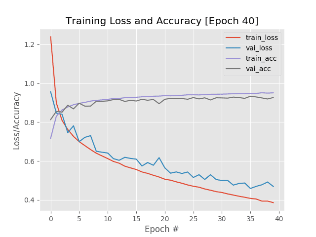
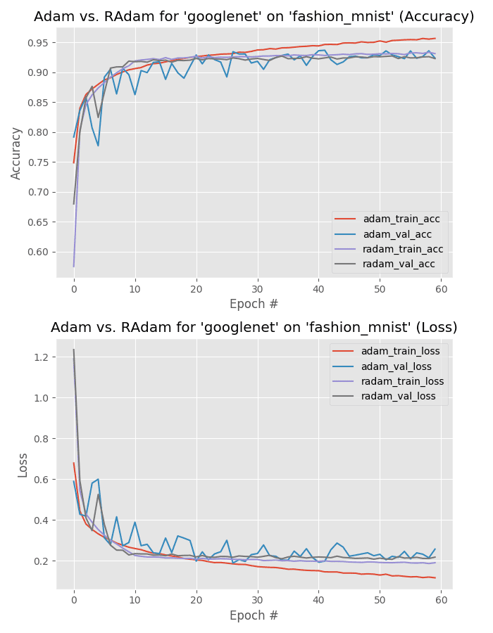
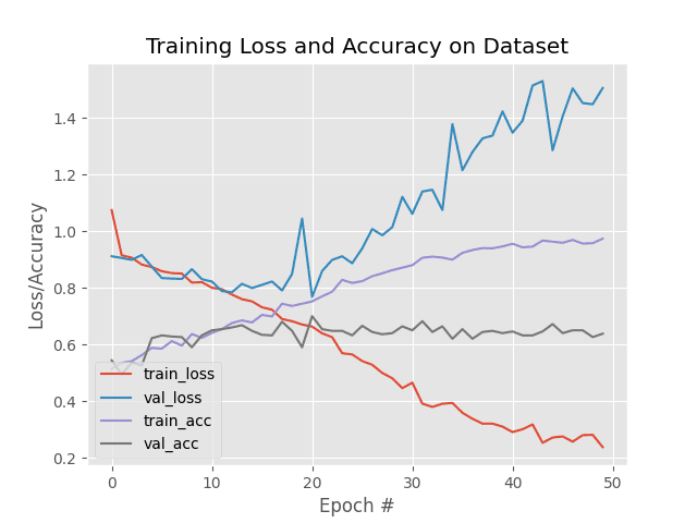
Figure 11: Is either RAdam or Adam a better deep learning optimizer using GoogLeNet? Using the Fashion MNIST dataset with Adam shows signs of overfitting past epoch 30. RAdam appears more stable in this experiment.
We now evaluate GoogLeNet trained on Fashion MNIST using Adam and Rectified Adam.
Below is the classification report from the Adam optimizer:
precision recall f1-score support
top 0.84 0.89 0.86 1000
trouser 1.00 0.99 0.99 1000
pullover 0.87 0.94 0.90 1000
dress 0.95 0.88 0.91 1000
coat 0.95 0.85 0.89 1000
sandal 0.98 0.99 0.98 1000
shirt 0.79 0.82 0.81 1000
sneaker 0.99 0.90 0.94 1000
bag 0.98 0.99 0.99 1000
ankle boot 0.91 0.99 0.95 1000
micro avg 0.92 0.92 0.92 10000
macro avg 0.93 0.92 0.92 10000
weighted avg 0.93 0.92 0.92 10000As well as the output from the Rectified Adam optimizer:
precision recall f1-score support
top 0.91 0.83 0.87 1000
trouser 0.99 0.99 0.99 1000
pullover 0.94 0.85 0.89 1000
dress 0.96 0.86 0.90 1000
coat 0.90 0.91 0.90 1000
sandal 0.98 0.98 0.98 1000
shirt 0.70 0.88 0.78 1000
sneaker 0.97 0.96 0.96 1000
bag 0.98 0.99 0.99 1000
ankle boot 0.97 0.97 0.97 1000
micro avg 0.92 0.92 0.92 10000
macro avg 0.93 0.92 0.92 10000
weighted avg 0.93 0.92 0.92 10000This time both optimizers obtain 93% accuracy, but what’s more interesting is to take a look at the training history plot in Figure 11.
Here we can see that training loss starts to diverge past epoch 30 for the Adam optimizer — this divergence grows wider and wider as we continue training. At this point, we should start to be concerned about overfitting using Adam.
On the other hand, Rectified Adam’s performance is stable with no signs of overfitting.
In this particular experiment, it’s clear that Rectified Adam is generalizing better, and had we wished to deploy this model to production, the Rectified Adam optimizer version would be the one to go with.
Fashion MNIST – ResNet
![]()
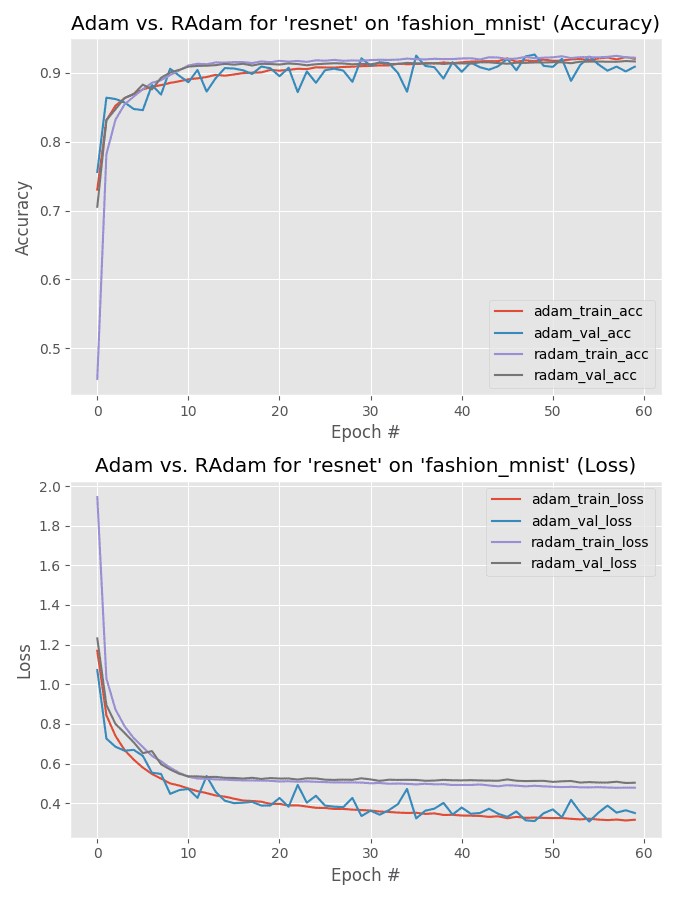
Figure 12: Which deep learning optimizer is better — Adam or Rectified Adam (RAdam) — using the ResNet CNN on the Fashion MNIST dataset?
Our final experiment compares Adam vs. Rectified Adam optimizer trained on the Fashion MNIST dataset using ResNet.
Below is the output of the Adam optimizer:
precision recall f1-score support
top 0.89 0.83 0.86 1000
trouser 0.99 0.99 0.99 1000
pullover 0.84 0.93 0.88 1000
dress 0.94 0.83 0.88 1000
coat 0.93 0.85 0.89 1000
sandal 0.99 0.92 0.95 1000
shirt 0.71 0.85 0.78 1000
sneaker 0.88 0.99 0.93 1000
bag 1.00 0.98 0.99 1000
ankle boot 0.98 0.93 0.95 1000
micro avg 0.91 0.91 0.91 10000
macro avg 0.92 0.91 0.91 10000
weighted avg 0.92 0.91 0.91 10000Here is the output of the Rectified Adam optimizer:
precision recall f1-score support
top 0.88 0.86 0.87 1000
trouser 0.99 0.99 0.99 1000
pullover 0.91 0.87 0.89 1000
dress 0.96 0.83 0.89 1000
coat 0.86 0.92 0.89 1000
sandal 0.98 0.98 0.98 1000
shirt 0.72 0.80 0.75 1000
sneaker 0.95 0.96 0.96 1000
bag 0.98 0.99 0.99 1000
ankle boot 0.97 0.96 0.96 1000
micro avg 0.92 0.92 0.92 10000
macro avg 0.92 0.92 0.92 10000
weighted avg 0.92 0.92 0.92 10000Both models obtain 92% accuracy, but take a look at the training history plot in Figure 12.
You can observe that Adam optimizer results in lower loss and that the validation loss follows the training curve.
The Rectified Adam loss is arguably more stable with fewer fluctuations (as compared to standard Adam).
Exactly which one is “better” in this experiment would be dependent on how well the model generalizes to images outside the training, validation, and testing set.
Further experiments would be required to mark the winner here, but my gut tells me that it’s Rectified Adam as (1) accuracy on the testing set is identical, and (2) lower loss doesn’t necessarily mean better generalization (in some cases it means that the model may fail to generalize well) — but at the same time, training/validation loss are near identical for Adam. Without further experiments it’s hard to make the call.
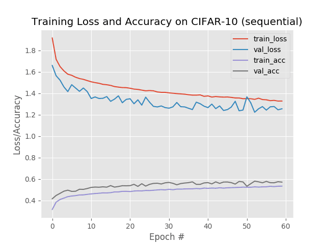
Adam vs. Rectified Adam Experiments with CIFAR-10
![]()
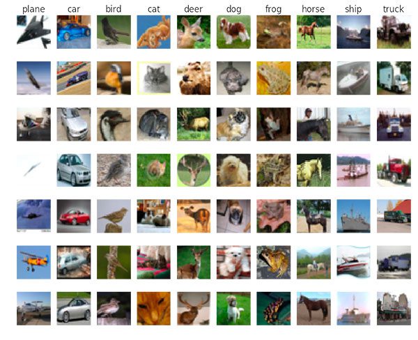
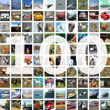
Figure 13: The CIFAR-10 benchmarking dataset has 10 classes. We will use it for Rectified Adam experimentation to evaluate if RAdam or Adam is the better choice (image source).
In these experiments, we’ll be comparing Adam vs. Rectified Adam performance using MiniVGGNet, GoogLeNet, and ResNet, all trained on the CIFAR-10 dataset.
CIFAR-10 – MiniVGGNet
![]()
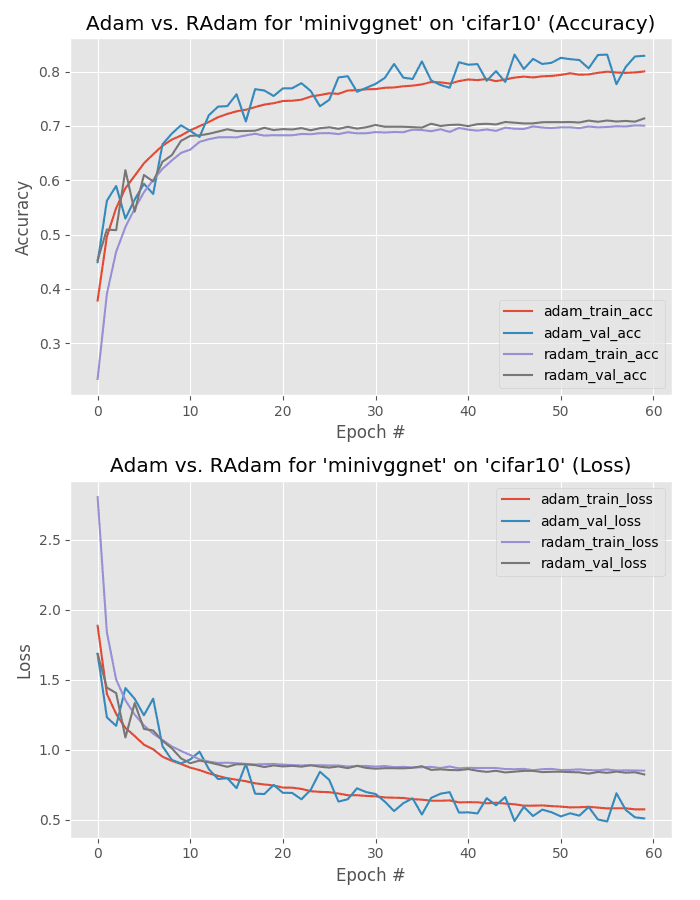
Figure 14: Is the RAdam or Adam deep learning optimizer better using the MiniVGGNet CNN on the CIFAR-10 dataset?
Our next experiment compares Adam to Rectified Adam by training MiniVGGNet on the CIFAR-10 dataset.
Below is the output of training using the Adam optimizer:
precision recall f1-score support
airplane 0.90 0.79 0.84 1000
automobile 0.90 0.93 0.91 1000
bird 0.90 0.63 0.74 1000
cat 0.78 0.68 0.73 1000
deer 0.83 0.79 0.81 1000
dog 0.81 0.76 0.79 1000
frog 0.70 0.95 0.81 1000
horse 0.85 0.91 0.88 1000
ship 0.93 0.89 0.91 1000
truck 0.77 0.95 0.85 1000
micro avg 0.83 0.83 0.83 10000
macro avg 0.84 0.83 0.83 10000
weighted avg 0.84 0.83 0.83 10000And here is the output from Rectified Adam:
precision recall f1-score support
airplane 0.84 0.72 0.78 1000
automobile 0.89 0.84 0.86 1000
bird 0.80 0.41 0.54 1000
cat 0.66 0.43 0.52 1000
deer 0.66 0.65 0.66 1000
dog 0.72 0.55 0.62 1000
frog 0.48 0.96 0.64 1000
horse 0.84 0.75 0.79 1000
ship 0.87 0.88 0.88 1000
truck 0.68 0.95 0.79 1000
micro avg 0.71 0.71 0.71 10000
macro avg 0.74 0.71 0.71 10000
weighted avg 0.74 0.71 0.71 10000Here the Adam optimizer (84% accuracy) beats out Rectified Adam (74% accuracy).
Furthermore, validation loss is lower than training loss for the majority of training, implying that we can “train harder” by reducing our regularization strength and potentially increasing model capacity.
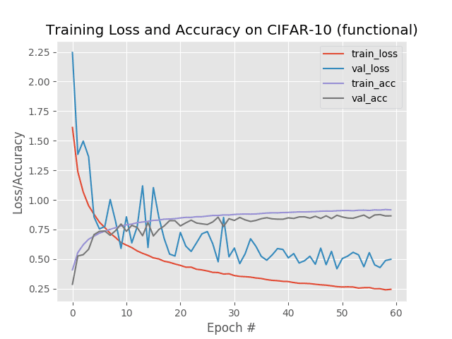
CIFAR-10 – GoogLeNet
![]()
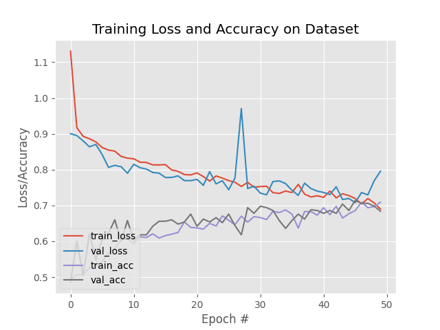
Figure 15: Which is a better deep learning optimizer with the GoogLeNet CNN? The training accuracy/loss plot shows results from using Adam and RAdam as part of automated deep learning experiment data collection.
Next, let’s check out GoogLeNet trained on CIFAR-10 using Adam and Rectified Adam.
Here is the output of Adam:
precision recall f1-score support
airplane 0.89 0.92 0.91 1000
automobile 0.92 0.97 0.94 1000
bird 0.90 0.87 0.88 1000
cat 0.79 0.86 0.82 1000
deer 0.92 0.85 0.89 1000
dog 0.92 0.81 0.86 1000
frog 0.87 0.96 0.91 1000
horse 0.95 0.91 0.93 1000
ship 0.96 0.92 0.94 1000
truck 0.90 0.94 0.92 1000
micro avg 0.90 0.90 0.90 10000
macro avg 0.90 0.90 0.90 10000
weighted avg 0.90 0.90 0.90 10000And here is the output of Rectified Adam:
precision recall f1-score support
airplane 0.88 0.88 0.88 1000
automobile 0.93 0.95 0.94 1000
bird 0.84 0.82 0.83 1000
cat 0.79 0.75 0.77 1000
deer 0.89 0.82 0.85 1000
dog 0.89 0.77 0.82 1000
frog 0.80 0.96 0.87 1000
horse 0.89 0.92 0.91 1000
ship 0.95 0.92 0.93 1000
truck 0.88 0.95 0.91 1000
micro avg 0.87 0.87 0.87 10000
macro avg 0.87 0.87 0.87 10000
weighted avg 0.87 0.87 0.87 10000The Adam optimizer obtains 90% accuracy, slightly beating out the 87% accuracy of Rectified Adam.
However, Figure 15 tells an interesting story — past epoch 20 there is quite the divergence between Adam’s training and validation loss.
While the Adam optimized model obtained higher accuracy, there are signs of overfitting as validation loss is essentially stagnant past epoch 30.
Additional experiments would be required to mark a true winner but I imagine it would be Rectified Adam after some additional hyperparameter tuning.
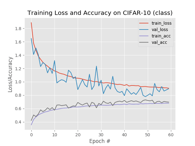
CIFAR-10 – ResNet
![]()
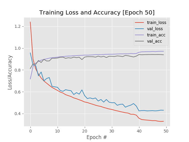
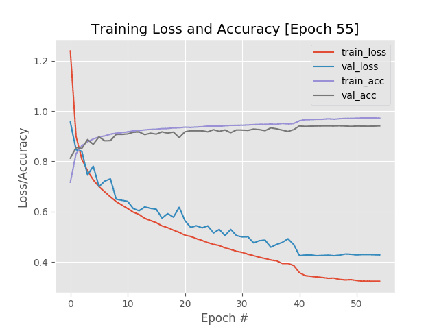
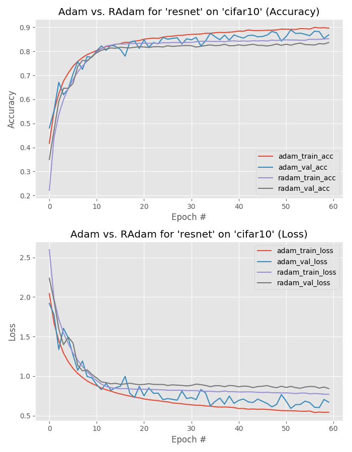
Figure 16: This Keras deep learning tutorial helps to answer the question: Is Rectified Adam or Adam the better deep learning optimizer? One of the 24 experiments uses the ResNet CNN and CIFAR-10 dataset.
Next, let’s check out ResNet trained using Adam and Rectified Adam on CIFAR-10.
Below you can find the output of the standard Adam optimizer:
precision recall f1-score support
airplane 0.80 0.92 0.86 1000
automobile 0.92 0.96 0.94 1000
bird 0.93 0.74 0.82 1000
cat 0.93 0.63 0.75 1000
deer 0.95 0.80 0.87 1000
dog 0.77 0.88 0.82 1000
frog 0.75 0.97 0.84 1000
horse 0.90 0.92 0.91 1000
ship 0.93 0.93 0.93 1000
truck 0.91 0.93 0.92 1000
micro avg 0.87 0.87 0.87 10000
macro avg 0.88 0.87 0.87 10000
weighted avg 0.88 0.87 0.87 10000As well as the output from Rectified Adam:
precision recall f1-score support
airplane 0.86 0.86 0.86 1000
automobile 0.89 0.95 0.92 1000
bird 0.85 0.72 0.78 1000
cat 0.78 0.66 0.71 1000
deer 0.83 0.81 0.82 1000
dog 0.82 0.70 0.76 1000
frog 0.72 0.95 0.82 1000
horse 0.86 0.90 0.87 1000
ship 0.94 0.90 0.92 1000
truck 0.84 0.93 0.88 1000
micro avg 0.84 0.84 0.84 10000
macro avg 0.84 0.84 0.83 10000
weighted avg 0.84 0.84 0.83 10000Adam is the winner here, obtaining 88% accuracy versus Rectified Adam’s 84%.
Adam vs. Rectified Adam Experiments with CIFAR-100
![]()
Figure 17: The CIFAR-100 classification dataset is the brother of CIFAR-10 and includes more classes of images. (image source)
The CIFAR-100 dataset is the bigger brother of the CIFAR-10 dataset. As the name suggests, CIFAR-100 includes 100 class labels versus the 10 class labels of CIFAR-10.
While there are more class labels in CIFAR-100, there are actually fewer images per class (CIFAR-10 has 6,000 images per class while CIFAR-100 only has 600 images per class).
CIFAR-100 is, therefore, a more challenging dataset than CIFAR-10.
In this section, we’ll investigate Adam vs. Rectified Adam’s performance on the CIFAR-100 dataset.
CIFAR-100 – MiniVGGNet
![]()
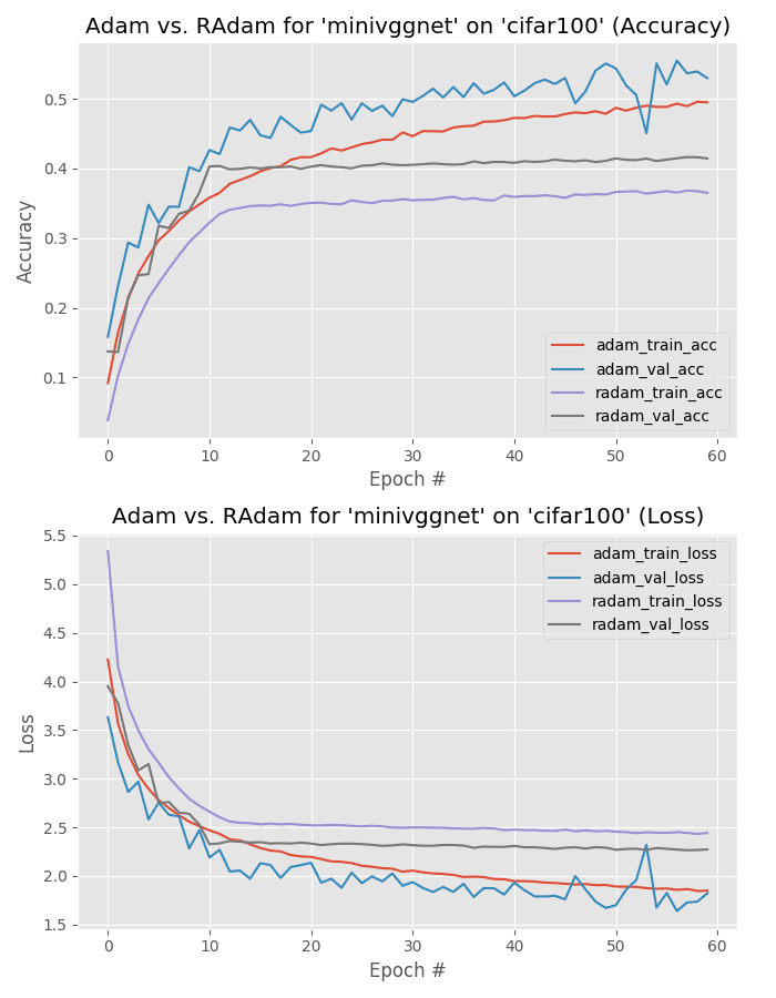
Figure 18: Will RAdam stand up to Adam as a preferable deep learning optimizer? How does Rectified Adam stack up to SGD? In this experiment (one of 24), we train MiniVGGNet on the CIFAR-100 dataset and analyze the results.
Let’s apply Adam and Rectified Adam to the MiniVGGNet architecture trained on CIFAR-100.
Below is the output from the Adam optimizer:
precision recall f1-score support
apple 0.94 0.76 0.84 100
aquarium_fish 0.69 0.66 0.67 100
baby 0.56 0.45 0.50 100
bear 0.45 0.22 0.30 100
beaver 0.31 0.14 0.19 100
bed 0.48 0.59 0.53 100
bee 0.60 0.69 0.64 100
beetle 0.51 0.49 0.50 100
bicycle 0.50 0.65 0.57 100
bottle 0.74 0.63 0.68 100
bowl 0.51 0.38 0.44 100
boy 0.45 0.37 0.41 100
bridge 0.64 0.68 0.66 100
bus 0.42 0.57 0.49 100
butterfly 0.52 0.50 0.51 100
camel 0.61 0.33 0.43 100
can 0.44 0.68 0.54 100
castle 0.74 0.71 0.72 100
caterpillar 0.78 0.40 0.53 100
cattle 0.58 0.48 0.52 100
chair 0.72 0.80 0.76 100
chimpanzee 0.74 0.64 0.68 100
clock 0.39 0.62 0.48 100
cloud 0.88 0.46 0.61 100
cockroach 0.80 0.66 0.73 100
couch 0.56 0.27 0.36 100
crab 0.43 0.52 0.47 100
crocodile 0.34 0.32 0.33 100
cup 0.74 0.73 0.73 100
..."d" - "t" classes omitted for brevity
wardrobe 0.67 0.87 0.76 100
whale 0.67 0.58 0.62 100
willow_tree 0.52 0.44 0.48 100
wolf 0.40 0.48 0.44 100
woman 0.39 0.19 0.26 100
worm 0.66 0.56 0.61 100
micro avg 0.53 0.53 0.53 10000
macro avg 0.58 0.53 0.53 10000
weighted avg 0.58 0.53 0.53 10000And here is the output from Rectified Adam:
precision recall f1-score support
apple 0.82 0.70 0.76 100
aquarium_fish 0.57 0.46 0.51 100
baby 0.55 0.26 0.35 100
bear 0.22 0.11 0.15 100
beaver 0.17 0.18 0.17 100
bed 0.47 0.37 0.42 100
bee 0.49 0.47 0.48 100
beetle 0.32 0.52 0.39 100
bicycle 0.36 0.64 0.46 100
bottle 0.74 0.40 0.52 100
bowl 0.47 0.29 0.36 100
boy 0.54 0.26 0.35 100
bridge 0.38 0.43 0.40 100
bus 0.34 0.35 0.34 100
butterfly 0.40 0.34 0.37 100
camel 0.37 0.19 0.25 100
can 0.57 0.45 0.50 100
castle 0.50 0.57 0.53 100
caterpillar 0.50 0.21 0.30 100
cattle 0.47 0.35 0.40 100
chair 0.54 0.72 0.62 100
chimpanzee 0.59 0.47 0.53 100
clock 0.29 0.37 0.33 100
cloud 0.77 0.60 0.67 100
cockroach 0.57 0.64 0.60 100
couch 0.42 0.18 0.25 100
crab 0.25 0.50 0.33 100
crocodile 0.30 0.28 0.29 100
cup 0.71 0.60 0.65 100
..."d" - "t" classes omitted for brevity
wardrobe 0.61 0.82 0.70 100
whale 0.57 0.39 0.46 100
willow_tree 0.36 0.27 0.31 100
wolf 0.32 0.39 0.35 100
woman 0.35 0.09 0.14 100
worm 0.62 0.32 0.42 100
micro avg 0.41 0.41 0.41 10000
macro avg 0.46 0.41 0.41 10000
weighted avg 0.46 0.41 0.41 10000The Adam optimizer is the clear winner (58% accuracy) over Rectified Adam (46% accuracy).
And just like in our CIFAR-10 experiments, we can likely improve our model performance further by relaxing regularization and increasing model capacity.
CIFAR-100 – GoogLeNet
![]()
Figure 19: Adam vs. RAdam optimizer on the CIFAR-100 dataset using GoogLeNet.
Let’s now perform the same experiment, only this time use GoogLeNet.
Here’s the output from the Adam optimizer:
precision recall f1-score support
apple 0.95 0.80 0.87 100
aquarium_fish 0.88 0.66 0.75 100
baby 0.59 0.39 0.47 100
bear 0.47 0.28 0.35 100
beaver 0.20 0.53 0.29 100
bed 0.79 0.56 0.65 100
bee 0.78 0.69 0.73 100
beetle 0.56 0.58 0.57 100
bicycle 0.91 0.63 0.75 100
bottle 0.80 0.71 0.75 100
bowl 0.46 0.37 0.41 100
boy 0.49 0.47 0.48 100
bridge 0.80 0.61 0.69 100
bus 0.62 0.60 0.61 100
butterfly 0.34 0.64 0.44 100
camel 0.93 0.37 0.53 100
can 0.42 0.69 0.52 100
castle 0.94 0.50 0.65 100
caterpillar 0.28 0.77 0.41 100
cattle 0.56 0.55 0.55 100
chair 0.85 0.77 0.81 100
chimpanzee 0.95 0.58 0.72 100
clock 0.56 0.62 0.59 100
cloud 0.88 0.68 0.77 100
cockroach 0.82 0.74 0.78 100
couch 0.66 0.40 0.50 100
crab 0.40 0.72 0.52 100
crocodile 0.36 0.47 0.41 100
cup 0.65 0.68 0.66 100
..."d" - "t" classes omitted for brevity
wardrobe 0.86 0.82 0.84 100
whale 0.40 0.80 0.53 100
willow_tree 0.46 0.62 0.53 100
wolf 0.86 0.37 0.52 100
woman 0.56 0.31 0.40 100
worm 0.79 0.57 0.66 100
micro avg 0.56 0.56 0.56 10000
macro avg 0.66 0.56 0.57 10000
weighted avg 0.66 0.56 0.57 10000And here is the output from Rectified Adam:
precision recall f1-score support
apple 0.93 0.76 0.84 100
aquarium_fish 0.72 0.77 0.74 100
baby 0.53 0.54 0.53 100
bear 0.47 0.26 0.34 100
beaver 0.26 0.22 0.24 100
bed 0.53 0.49 0.51 100
bee 0.52 0.62 0.56 100
beetle 0.50 0.55 0.52 100
bicycle 0.67 0.79 0.72 100
bottle 0.78 0.62 0.69 100
bowl 0.41 0.42 0.41 100
boy 0.45 0.41 0.43 100
bridge 0.59 0.72 0.65 100
bus 0.45 0.53 0.49 100
butterfly 0.27 0.58 0.37 100
camel 0.56 0.50 0.53 100
can 0.58 0.68 0.63 100
castle 0.81 0.73 0.77 100
caterpillar 0.51 0.52 0.51 100
cattle 0.56 0.59 0.58 100
chair 0.68 0.76 0.72 100
chimpanzee 0.83 0.73 0.78 100
clock 0.46 0.56 0.50 100
cloud 0.88 0.69 0.78 100
cockroach 0.79 0.68 0.73 100
couch 0.44 0.39 0.41 100
crab 0.46 0.47 0.46 100
crocodile 0.40 0.40 0.40 100
cup 0.76 0.62 0.68 100
..."d" - "t" classes omitted for brevity
wardrobe 0.76 0.87 0.81 100
whale 0.56 0.61 0.59 100
willow_tree 0.65 0.30 0.41 100
wolf 0.61 0.55 0.58 100
woman 0.39 0.30 0.34 100
worm 0.62 0.61 0.62 100
micro avg 0.57 0.57 0.57 10000
macro avg 0.59 0.57 0.57 10000
weighted avg 0.59 0.57 0.57 10000The Adam optimizer obtains 66% accuracy, better than Rectified Adam’s 59%.
However, looking at Figure 19 we can see that the validation loss from Adam is quite unstable — towards the end of training validation loss even starts to increase, a sign of overfitting.
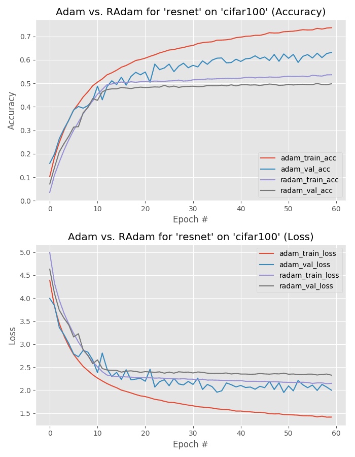
CIFAR-100 – ResNet
![]()
Figure 20: Training a ResNet model on the CIFAR-100 dataset using both RAdam and Adam for comparison. Which deep learning optimizer is actually better for this experiment?
Below we can find the output of training ResNet using Adam on the CIFAR-100 dataset:
precision recall f1-score support
apple 0.80 0.89 0.84 100
aquarium_fish 0.86 0.75 0.80 100
baby 0.75 0.40 0.52 100
bear 0.71 0.29 0.41 100
beaver 0.40 0.40 0.40 100
bed 0.91 0.59 0.72 100
bee 0.71 0.76 0.73 100
beetle 0.82 0.42 0.56 100
bicycle 0.54 0.89 0.67 100
bottle 0.93 0.62 0.74 100
bowl 0.75 0.36 0.49 100
boy 0.43 0.49 0.46 100
bridge 0.54 0.78 0.64 100
bus 0.68 0.48 0.56 100
butterfly 0.34 0.71 0.46 100
camel 0.72 0.68 0.70 100
can 0.69 0.60 0.64 100
castle 0.96 0.69 0.80 100
caterpillar 0.57 0.62 0.60 100
cattle 0.91 0.51 0.65 100
chair 0.79 0.82 0.80 100
chimpanzee 0.80 0.79 0.79 100
clock 0.41 0.86 0.55 100
cloud 0.89 0.74 0.81 100
cockroach 0.85 0.78 0.81 100
couch 0.73 0.44 0.55 100
crab 0.42 0.70 0.53 100
crocodile 0.47 0.55 0.51 100
cup 0.88 0.75 0.81 100
..."d" - "t" classes omitted for brevity
wardrobe 0.79 0.85 0.82 100
whale 0.58 0.75 0.65 100
willow_tree 0.71 0.37 0.49 100
wolf 0.79 0.64 0.71 100
woman 0.42 0.49 0.45 100
worm 0.48 0.80 0.60 100
micro avg 0.63 0.63 0.63 10000
macro avg 0.68 0.63 0.63 10000
weighted avg 0.68 0.63 0.63 10000And here is the output of Rectified Adam:
precision recall f1-score support
apple 0.86 0.72 0.78 100
aquarium_fish 0.56 0.62 0.59 100
baby 0.49 0.43 0.46 100
bear 0.36 0.20 0.26 100
beaver 0.27 0.17 0.21 100
bed 0.45 0.42 0.43 100
bee 0.54 0.61 0.57 100
beetle 0.47 0.55 0.51 100
bicycle 0.45 0.69 0.54 100
bottle 0.64 0.54 0.59 100
bowl 0.39 0.31 0.35 100
boy 0.43 0.35 0.38 100
bridge 0.52 0.67 0.59 100
bus 0.34 0.47 0.40 100
butterfly 0.33 0.39 0.36 100
camel 0.47 0.37 0.41 100
can 0.49 0.55 0.52 100
castle 0.76 0.67 0.71 100
caterpillar 0.43 0.43 0.43 100
cattle 0.56 0.45 0.50 100
chair 0.63 0.78 0.70 100
chimpanzee 0.70 0.71 0.71 100
clock 0.38 0.49 0.43 100
cloud 0.80 0.61 0.69 100
cockroach 0.73 0.72 0.73 100
couch 0.49 0.36 0.42 100
crab 0.27 0.45 0.34 100
crocodile 0.32 0.26 0.29 100
cup 0.63 0.49 0.55 100
..."d" - "t" classes omitted for brevity
wardrobe 0.68 0.84 0.75 100
whale 0.53 0.54 0.54 100
willow_tree 0.60 0.29 0.39 100
wolf 0.38 0.35 0.36 100
woman 0.33 0.29 0.31 100
worm 0.59 0.63 0.61 100
micro avg 0.50 0.50 0.50 10000
macro avg 0.51 0.50 0.49 10000
weighted avg 0.51 0.50 0.49 10000The Adam optimizer (68% accuracy) crushes Rectified Adam (51% accuracy) here, but we need to be careful of overfitting. As Figure 20 shows there is quite the divergence between training and validation loss when using the Adam optimizer.
But on the other hand, Rectified Adam really stagnates past epoch 20.
I would be inclined to go with the Adam optimized model here as it obtains significantly higher accuracy; however, I would suggest running some generalization tests using both the Adam and Rectified Adam versions of the model.
What can we take away from these experiments?
One of the first takeaways comes from looking at the training plots of the experiments — using the Rectified Adam optimizer can lead to more stable training.
When training with Rectified Adam we see there are significantly fewer fluctuations, spikes, and drops in validation loss (as compared to standard Adam).
Furthermore, the Rectified Adam validation loss is much more likely to follow training loss, in some cases near exactly.
Keep in mind that raw accuracy isn’t everything when it comes to training your own custom neural networks — stability matters as well as it goes hand-in-hand with generalization.
Whenever I’m training a custom CNN I’m not only looking for high accuracy models, I’m also looking for stability. Stability typically implies that a model is converging nicely and will ideally generalize well.
In this regard, Rectified Adam delivers on its promises from the Liu et al. paper.
Secondly, you should note that Adam obtains lower loss than Rectified Adam in every single experiment.
This behavior is not necessarily a bad thing — it could imply that Rectified Adam is generalizing better, but it’s hard to say without running further experiments using images outside the respective training and testing sets.
Again, keep in mind that lower loss is not necessarily a better model! When you encounter very low loss (especially loss near zero) your model may be overfitting to your training set.
You need to obtain mastery level experience operating these three optimizers
![]()
Figure 21: Mastering deep learning optimizers is like driving a car. You know your car and you drive it well no matter the road condition. On the other hand, if you get in an unfamiliar car, something doesn’t feel right until you have a few hours cumulatively behind the wheel. Optimizers are no different. I suggest that SGD be your daily driver until you are comfortable trying alternatives. Then you can mix in RMSprop and Adam. Learn how to use them before jumping into the latest deep learning optimizer.
Becoming familiar with a given optimization algorithm is similar to mastering how to drive a car — you drive your own car better than other people’s cars because you’ve spent so much time driving it; you understand your car and its intricacies.
Often times, a given optimizer is chosen to train a network on a dataset not because the optimizer itself is better, but because the driver (i.e., you, the deep learning practitioner) is more familiar with the optimizer and understands the “art” behind tuning its respective parameters.
As a deep learning practitioner you should gain experience operating a wide variety of optimizers, but in my opinion, you should focus your efforts on learning how to train networks using the three following optimizers:
- SGD
- RMSprop
- Adam
You might be surprised to see SGD is included in this list — isn’t SGD an older, less efficient optimizer than the newer adaptive methods, including Adam, Adagrad, Adadelta, etc.?
Yes, it absolutely is.
But here’s the thing — nearly every state-of-the-art computer vision model is trained using SGD.
Consider the ImageNet classification challenge for example:
- AlexNet (there’s no mention in the paper but both the official implementation and CaffeNet used SGD)
- VGGNet (Section 3.1, Training)
- ResNet (Section 3.4, Implementation)
- SqueezeNet (it’s not mentioned in the paper, but SGD was used in their solver.prototxt)
Every single one of those classification networks was trained using SGD.
Now let’s consider the object detection networks trained on the COCO dataset:
You guessed it — SGD was used to train all of them.
Yes, SGD may the “old, unsexy” optimizer compared to its younger counterparts, but here’s the thing, standard SGD just works.
That’s not to say that you shouldn’t learn how to use other optimizers — you absolutely should!
But before you go down that rabbit hole, obtain a mastery level of SGD first. From there, start exploring other optimizers — I typically recommend RMSprop and Adam.
And if you find Adam is working well, consider replacing Adam with Rectified Adam to see if you can get an additional boost in accuracy (sort of like how replacing ReLUs with ELUs can usually give you a small boost).
Once you understand how to use those optimizers on a variety of datasets, continue your studies and explore other optimizers as well.
All that said, if you’re new to deep learning, don’t immediately try jumping into the more “advanced” optimizers — you’ll only run into trouble later in your deep learning career.
What’s next?
If you’re interested in diving head-first into the world of computer vision/deep learning and discovering how to:
- Understand, practice, and proficiently operate each of the “big three” optimizers
- Select the best optimizer for the job to achieve state-of-the-art results
- Train custom Convolutional Neural Networks on your own custom datasets
- Learn my best practices, tips, and suggestions (leading you to becoming a deep learning expert)
…then be sure to take a look at my book, Deep Learning for Computer Vision with Python!
My complete, self-study deep learning book is trusted by members of top machine learning schools, companies, and organizations, including Microsoft, Google, Stanford, MIT, CMU, and more!
Readers of my book have gone on to win Kaggle competitions, secure academic grants, and start careers in CV and DL using the knowledge they gained through study and practice.
My book not only teaches the fundamentals, but also teaches advanced techniques, best practices, and tools to ensure that you are armed with practical knowledge and proven coding recipes to tackle nearly any computer vision and deep learning problem presented to you in school, research, or the modern workforce.
Be sure to take a look — and while you’re at it, don’t forget to grab your (free) table of contents + sample chapters.
Summary
In this tutorial, we investigated the claims from Liu et al. that the Rectified Adam optimizer outperforms the standard Adam optimizer in terms of:
- Better accuracy (or at least identical accuracy when compared to Adam)
- And in fewer epochs than standard Adam
To evaluate those claims we trained three CNN models:
- ResNet
- GoogLeNet
- MiniVGGNet
These models were trained on four datasets:
- MNIST
- Fashion MNIST
- CIFAR-10
- CIFAR-100
Each combination of the model architecture and dataset were trained using two optimizers:
In total, we ran 3 x 4 x 2 = 24 different experiments used to compare standard Adam to Rectified Adam.
The result?
In each and every experiment Rectified Adam either performed worse or obtained identical accuracy compared to standard Adam.
That said, training with Rectified Adam was more stable than standard Adam, likely implying that Rectified Adam could generalize better (but additional experiments would be required to validate that claim).
Liu et al.’s study of warmup can be utilized in adaptive learning rate optimizers and will likely help future researchers build on their work and create even better optimizers.
For the time being, my personal opinion is that you’re better off sticking with standard Adam for your initial experiments. If you find that Adam is working well for your experiments, substitute in Rectified Adam to see if you can improve your accuracy.
You should especially try to use the Rectified Adam optimizer if you notice that Adam is working well, but you need better generalization.
The second takeaway from this guide is that you should obtain mastery level experience operating these three optimizers:
- SGD
- RMSprop
- Adam
You should especially learn how to operate SGD.
Yes, SGD is “less sexy” compared to the newer adaptive learning rate methods, but nearly every computer vision state-of-the-art architecture has been trained using it.
Learn how to operate these three optimizers first.
Once you have a good understanding of how they work and how to tune their respective hyperparameters, then move on to other optimizers.
If you need help learning how to use these optimizers and tune their hyperparameters, be sure to refer to Deep Learning for Computer Vision with Python where I cover my tips, suggestions, and best practices in detail.
To download the source code to this post (and be notified when future tutorials are published here on PyImageSearch), just enter your email address in the form below!
Downloads:
The post Is Rectified Adam actually *better* than Adam? appeared first on PyImageSearch.


 drawn from a random distribution (right).


 – Match 27

 , controls the “step” we make along the gradient. Larger values of
  .
.
 steps per epoch. Therefore, a total of
  and our
  (with the assumption that we are training for forty epochs).
} = 0.01")
} = 0.00836")
 and a decay of
  :
:
 .
. , etc.
 / D}")
 is the initial learning rate,
  is the factor value controlling the rate in which the learning date drops, D is the “Drop every” epochs value, and E is the current epoch.