Quantcast
Channel: Tutorials Archives - PyImageSearch
Viewing all 432 articles
Browse latest View live

How to configure your NVIDIA Jetson Nano for Computer Vision and Deep Learning

$
0
0

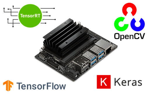
In today’s tutorial, you will learn how to configure your NVIDIA Jetson Nano for Computer Vision and Deep Learning with TensorFlow, Keras, TensorRT, and OpenCV.

Two weeks ago, we discussed how to use my pre-configured Nano .img filetoday, you will learn how to configure your own Nano from scratch.

This guide requires you to have at least 48 hours of time to kill as you configure your NVIDIA Jetson Nano on your own (yes, it really is that challenging)

If you decide you want to skip the hassle and use my pre-configured Nano .img, you can find it as part of my brand-new book, Raspberry Pi for Computer Vision.

But for those brave enough to go through the gauntlet, this post is for you!

To learn how to configure your NVIDIA Jetson Nano for computer vision and deep learning, just keep reading.

Looking for the source code to this post?

Jump Right To The Downloads Section

How to configure your NVIDIA Jetson Nano for Computer Vision and Deep Learning

The NVIDIA Jetson Nano packs 472GFLOPS of computational horsepower. While it is a very capable machine, configuring it is not (complex machines are typically not easy to configure).

In this tutorial, we’ll work through 16 steps to configure your Jetson Nano for computer vision and deep learning.

Prepare yourself for a long, grueling process — you may need 2-5 days of your time to configure your Nano following this guide.

Once we are done, we will test our system to ensure it is configured properly and that TensorFlow/Keras and OpenCV are operating as intended. We will also test our Nano’s camera with OpenCV to ensure that we can access our video stream.

If you encounter a problem with the final testing step, then you may need to go back and resolve it; or worse, start back at the very first step and endure another 2-5 days of pain and suffering through the configuration tutorial to get up and running (but don’t worry, I present an alternative at the end of the 16 steps).

Step #1: Flash NVIDIA’s Jetson Nano Developer Kit .img to a microSD for Jetson Nano

In this step, we will download NVIDIA’s Jetpack 4.2 Ubuntu-based OS image and flash it to a microSD. You will need the microSD flashed and ready to go to follow along with the next steps.

Go ahead and start your download here, ensuring that you download the “Jetson Nano Developer Kit SD Card image” as shown in the following screenshot:

Figure 1: The first step to configure your NVIDIA Jetson Nano for computer vision and deep learning is to download the Jetpack SD card image.

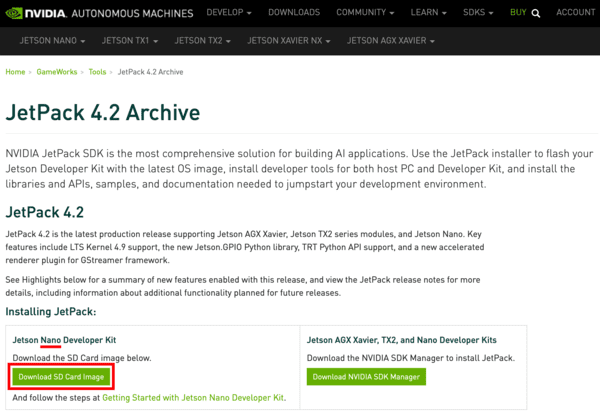
We recommend the Jetpack 4.2 for compatibility with the Complete Bundle of Raspberry Pi for Computer Vision (our recommendation will inevitably change in the future).

While your Nano SD image is downloading, go ahead and download and install balenaEtcher, a disk image flashing tool:

Figure 2: Download and install balenaEtcher for your OS. You will use it to flash your Nano image to a microSD card.

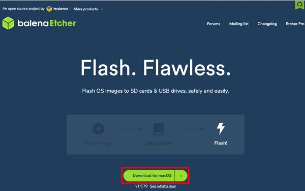
Once both (1) your Nano Jetpack image is downloaded, and (2) balenaEtcher is installed, you are ready to flash the image to a microSD.

You will need a suitable microSD card and microSD reader hardware. We recommend either a 32GB or 64GB microSD card (SanDisk’s 98MB/s cards are high quality, and Amazon carries them if they are a distributor in your locale). Any microSD card reader should work.

Insert the microSD into the card reader, and then plug the card reader into a USB port on your computer. From there, fire up balenaEtcher and proceed to flash.

Figure 3: Flashing NVIDIA’s Jetpack image to a microSD card with balenaEtcher is one of the first steps for configuring your Nano for computer vision and deep learning.

When flashing has successfully completed, you are ready to move on to Step #2.

Step #2: Boot your Jetson Nano with the microSD and connect to a network

Figure 4: The NVIDIA Jetson Nano does not come with WiFi capability, but you can use a USB WiFi module (top-right) or add a more permanent module under the heatsink (bottom-center). Also pictured is a 5V 4A (20W) power supply (top-left) that you may wish to use to power your Jetson Nano if you have lots of hardware attached to it.

In this step, we will power up our Jetson Nano and establish network connectivity.

This step requires the following:

  1. The flashed microSD from Step #1
  2. An NVIDIA Jetson Nano dev board
  3. HDMI screen
  4. USB keyboard + mouse
  5. A power supply — either (1) a 5V 2.5A (12.5W) microSD power supply or (2) a 5V 4A (20W) barrel plug power supply with a jumper at the J48 connector
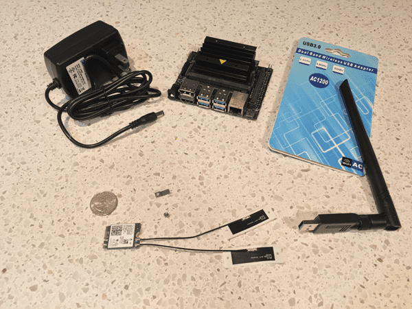
  6. Network connection — either (1) an Ethernet cable connecting your Nano to your network or (2) a wireless module. The wireless module can come in the form of a USB WiFi adapter or a WiFi module installed under the Jetson Nano heatsink

If you want WiFi (most people do), you must add a WiFi module on your own. Two great options for adding WiFi to your Jetson Nano include:

  • USB to WiFi adapter (Figure 4top-right). No tools are required and it is portable to other devices. Pictured is the Geekworm Dual Band USB 1200m
  • WiFi module such as the Intel Dual Band Wireless-Ac 8265 W/Bt (Intel 8265NGW) and 2x Molex Flex 2042811100 Flex Antennas (Figure 5, bottom-center). You must install the WiFi module and antennas under the main heatsink on your Jetson Nano. This upgrade requires a Phillips #2 screwdriver, the wireless module, and antennas (not to mention about 10-20 minutes of your time)

We recommend going with a USB WiFi adapter if you need to use WiFi with your Jetson Nano. There are many options available online, so try to purchase one that has Ubuntu 18.04 drivers preinstalled on the OS so that you don’t need to scramble to download and install drivers as we did following these instructions for the Geekworm product (it could be tough if you don’t have a wired connection available in the first place to download and install the drivers).

Once you have gathered all the gear, insert your microSD into your Jetson Nano as shown in Figure 5:

Figure 5: To insert your Jetpack-flashed microSD after it has been flashed, find the microSD slot as shown by the red circle in the image. Insert your microSD until it clicks into place.

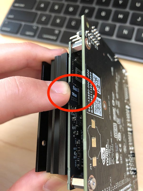
From there, connect your screen, keyboard, mouse, and network interface.

Finally, apply power. Insert the power plug of your power adapter into your Jetson Nano (use the J48 jumper if you are using a 20W barrel plug supply).

Figure 6: Use the icon near the top right corner of your screen to configure networking settings on your NVIDIA Jetson Nano. You will need internet access to download and install computer vision and deep learning software.

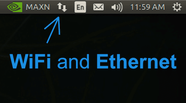
Once you see your NVIDIA + Ubuntu 18.04 desktop, you should configure your wired or wireless network settings as needed using the icon in the menubar as shown in Figure 6.

When you have confirmed that you have internet access on your NVIDIA Jetson Nano, you can move on to the next step.

Step #3: Open a terminal or start an SSH session

In this step we will do one of the following:

  1. Option 1: Open a terminal on the Nano desktop, and assume that you’ll perform all steps from here forward using the keyboard and mouse connected to your Nano
  2. Option 2: Initiate an SSH connection from a different computer so that we can remotely configure our NVIDIA Jetson Nano for computer vision and deep learning

Both options are equally good.

Option 1: Use the terminal on your Nano desktop

For Option 1, open up the application launcher, and select the terminal app. You may wish to right click it in the left menu and lock it to the launcher, since you will likely use it often.

You may now continue to Step #4 while keeping the terminal open to enter commands.

Option 2: Initiate an SSH remote session

For Option 2, you must first determine the username and IP address of your Jetson Nano. On your Nano, fire up a terminal from the application launcher, and enter the following commands at the prompt:

$ whoami
nvidia
$ ifconfig
en0: flags=8863 mtu 1500
	options=400
	ether 8c:85:90:4f:b4:41
	inet6 fe80::14d6:a9f6:15f8:401%en0 prefixlen 64 secured scopeid 0x8
	inet6 2600:100f:b0de:1c32:4f6:6dc0:6b95:12 prefixlen 64 autoconf secured
	inet6 2600:100f:b0de:1c32:a7:4e69:5322:7173 prefixlen 64 autoconf temporary
	inet 192.168.1.4 netmask 0xffffff00 broadcast 192.168.1.255
	nd6 options=201
	media: autoselect
	status: active

Grab your IP address (it is on the highlighted line). My IP address is 192.168.1.4; however, your IP address will be different, so make sure you check and verify your IP address!

Then, on a separate computer, such as your laptop/desktop, initiate an SSH connection as follows:

$ ssh nvidia@192.168.1.4

Notice how I’ve entered the username and IP address of the Jetson Nano in my command to remotely connect. You should now have a successful connection to your Jetson Nano, and you can continue on with Step #4.

Step #4: Update your system and remove programs to save space

In this step, we will remove programs we don’t need and update our system.

First, let’s set our Nano to use maximum power capacity:

$ sudo nvpmodel -m 0
$ sudo jetson_clocks

The nvpmodel command handles two power options for your Jetson Nano: (1) 5W is mode 1 and (2) 10W is mode 0. The default is the higher wattage mode, but it is always best to force the mode before running the jetson_clocks command.

According to the NVIDIA devtalk forums:

The jetson_clocks script disables the DVFS governor and locks the clocks to their maximums as defined by the active nvpmodel power mode. So if your active mode is 10W, jetson_clocks will lock the clocks to their maximums for 10W mode. And if your active mode is 5W, jetson_clocks will lock the clocks to their maximums for 5W mode (NVIDIA DevTalk Forums).

Note: There are two typical ways to power your Jetson Nano. A 5V 2.5A (10W) microUSB power adapter is a good option. If you have a lot of gear being powered by the Nano (keyboards, mice, WiFi, cameras), then you should consider a 5V 4A (20W) power supply to ensure that your processors can run at their full speeds while powering your peripherals. Technically there’s a third power option too if you want to apply power directly on the header pins.

After you have set your Nano for maximum power, go ahead and remove LibreOffice — it consumes lots of space, and we won’t need it for computer vision and deep learning:

$ sudo apt-get purge libreoffice*
$ sudo apt-get clean

From there, let’s go ahead and update system level packages:

$ sudo apt-get update && sudo apt-get upgrade

In the next step, we’ll begin installing software.

Step #5: Install system-level dependencies

The first set of software we need to install includes a selection of development tools:

$ sudo apt-get install git cmake
$ sudo apt-get install libatlas-base-dev gfortran
$ sudo apt-get install libhdf5-serial-dev hdf5-tools
$ sudo apt-get install python3-dev
$ sudo apt-get install nano locate

Next, we’ll install SciPy prerequisites (gathered from NVIDIA’s devtalk forums) and a system-level Cython library:

$ sudo apt-get install libfreetype6-dev python3-setuptools
$ sudo apt-get install protobuf-compiler libprotobuf-dev openssl
$ sudo apt-get install libssl-dev libcurl4-openssl-dev
$ sudo apt-get install cython3

We also need a few XML tools for working with TensorFlow Object Detection (TFOD) API projects:

$ sudo apt-get install libxml2-dev libxslt1-dev

Step #6: Update CMake

Now we’ll update the CMake precompiler tool as we need a newer version in order to successfully compile OpenCV.

First, download and extract the CMake update:

$ wget http://www.cmake.org/files/v3.13/cmake-3.13.0.tar.gz
$ tar xpvf cmake-3.13.0.tar.gz cmake-3.13.0/

Next, compile CMake:

$ cd cmake-3.13.0/
$ ./bootstrap --system-curl
$ make -j8

And finally, update your bash profile:

$ echo 'export PATH=/home/nvidia/cmake-3.13.0/bin/:$PATH' >> ~/.bashrc
$ source ~/.bashrc

CMake is now ready to go on your system. Ensure that you do not delete the cmake-3.13.0/ directory in your home folder.

Step #7: Install OpenCV system-level dependencies and other development dependencies

Let’s now install OpenCV dependecies on our system beginning with tools needed to build and compile OpenCV with parallelism:

$ sudo apt-get install build-essential pkg-config
$ sudo apt-get install libtbb2 libtbb-dev

Next, we’ll install a handful of codecs and image libraries:

$ sudo apt-get install libavcodec-dev libavformat-dev libswscale-dev
$ sudo apt-get install libxvidcore-dev libavresample-dev
$ sudo apt-get install libtiff-dev libjpeg-dev libpng-dev

And then we’ll install a selection of GUI libraries:

$ sudo apt-get install python-tk libgtk-3-dev
$ sudo apt-get install libcanberra-gtk-module libcanberra-gtk3-module

Lastly, we’ll install Video4Linux (V4L) so that we can work with USB webcams and install a library for FireWire cameras:

$ sudo apt-get install libv4l-dev libdc1394-22-dev

Step #8: Set up Python virtual environments on your Jetson Nano

Figure 7: Each Python virtual environment you create on your NVIDIA Jetson Nano is separate and independent from the others.

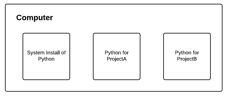
I can’t stress this enough: Python virtual environments are a best practice when both developing and deploying Python software projects.

Virtual environments allow for isolated installs of different Python packages. When you use them, you could have one version of a Python library in one environment and another version in a separate, sequestered environment.

In the remainder of this tutorial, we’ll create one such virtual environment; however, you can create multiple environments for your needs after you complete this Step #8. Be sure to read the RealPython guide on virtual environments if you aren’t familiar with them.

First, we’ll install the de facto Python package management tool, pip:

$ wget https://bootstrap.pypa.io/get-pip.py
$ sudo python3 get-pip.py
$ rm get-pip.py

And then we’ll install my favorite tools for managing virtual environments, virtualenv and virtualenvwrapper:

$ sudo pip install virtualenv virtualenvwrapper

The virtualenvwrapper tool is not fully installed until you add information to your bash profile. Go ahead and open up your ~/.bashrc with the nano ediitor:

$ nano ~/.bashrc

And then insert the following at the bottom of the file:

# virtualenv and virtualenvwrapper
export WORKON_HOME=$HOME/.virtualenvs
export VIRTUALENVWRAPPER_PYTHON=/usr/bin/python3
source /usr/local/bin/virtualenvwrapper.sh

Save and exit the file using the keyboard shortcuts shown at the bottom of the nano editor, and then load the bash profile to finish the virtualenvwrapper installation:

$ source ~/.bashrc
Figure 8: Terminal output from the virtualenvwrapper setup installation indicates that there are no errors. We now have a virtual environment management system in place so we can create computer vision and deep learning virtual environments on our NVIDIA Jetson Nano.

So long as you don’t encounter any error messages, both virtualenv and virtualenvwrapper are now ready for you to create and destroy virtual environments as needed in Step #9.

Step #9: Create your ‘py3cv4’ virtual environment

This step is dead simple once you’ve installed virtualenv and virtualenvwrapper in the previous step. The virtualenvwrapper tool provides the following commands to work with virtual environments:

  • mkvirtualenv: Create a Python virtual environment
  • lsvirtualenv: List virtual environments installed on your system
  • rmvirtualenv: Remove a virtual environment
  • workon: Activate a Python virtual environment
  • deactivate: Exits the virtual environment taking you back to your system environment

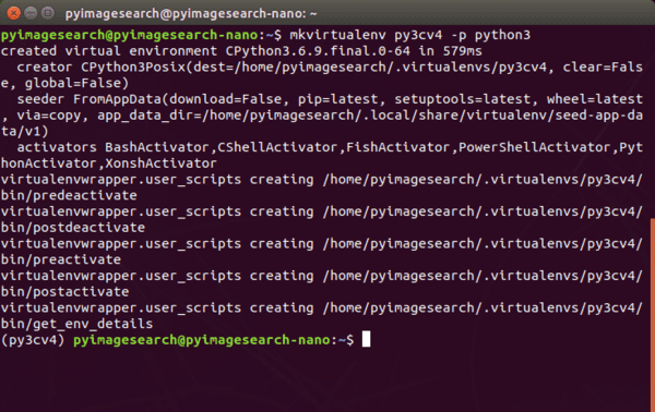
Assuming Step #8 went smoothly, let’s create a Python virtual environment on our Nano:

$ mkvirtualenv py3cv4 -p python3

I’ve named the virtual environment py3cv4 indicating that we will use Python 3 and OpenCV 4. You can name yours whatever you’d like depending on your project and software needs or even your own creativity.

When your environment is ready, your bash prompt will be preceded by (py3cv4). If your prompt is not preceded by the name of your virtual environment name, at any time you can use the workon command as follows:

$ workon py3cv4
Figure 9: Ensure that your bash prompt begins with your virtual environment name for the remainder of this tutorial on configuring your NVIDIA Jetson Nano for deep learning and computer vision.

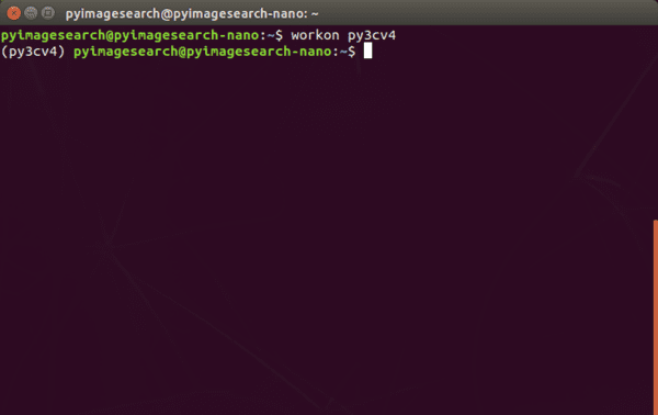
For the remaining steps in this tutorial, you must be “in” the py3cv4 virtual environment.

Step #10: Install the Protobuf Compiler

This section walks you through the step-by-step process for configuring protobuf so that TensorFlow will be fast.

TensorFlow’s performance can be significantly impacted (in a negative way) if an efficient implementation of protobuf and libprotobuf are not present.

When we pip-install TensorFlow, it automatically installs a version of protobuf that might not be the ideal one. The issue with slow TensorFlow performance has been detailed in this NVIDIA Developer forum.

First, download and install an efficient implementation of the protobuf compiler (source):

$ wget https://raw.githubusercontent.com/jkjung-avt/jetson_nano/master/install_protobuf-3.6.1.sh
$ sudo chmod +x install_protobuf-3.6.1.sh
$ ./install_protobuf-3.6.1.sh

This will take approximately one hour to install, so go for a nice walk, or read a good book such as Raspberry Pi for Computer Vision or Deep Learning for Computer Vision with Python.

Once protobuf is installed on your system, you need to install it inside your virtual environment:

$ workon py3cv4 # if you aren't inside the environment
$ cd ~
$ cp -r ~/src/protobuf-3.6.1/python/ .
$ cd python
$ python setup.py install --cpp_implementation

Notice that rather than using pip to install the protobuf package, we used a setup.py installation script. The benefit of using setup.py is that we compile software specifically for the Nano processor rather than using generic precompiled binaries.

In the remaining steps we will use a mix of setup.py (when we need to optimize a compile) and pip (when the generic compile is sufficient).

Let’s move on to Step #11 where we’ll install deep learning software.

Step #11: Install TensorFlow, Keras, NumPy, and SciPy on Jetson Nano

In this section, we’ll install TensorFlow/Keras and their dependencies.

First, ensure you’re in the virtual environment:

$ workon py3cv4

And then install NumPy and Cython:

$ pip install numpy cython

You may encounter the following error message:

ERROR: Could not build wheels for numpy which use PEP 517 and cannot be installed directly.

If you come across that message, then follow these additional steps. First, install NumPy with super user privileges:

$ sudo pip install numpy

Then, create a symbolic link from your system’s NumPy into your virtual environment site-packages. To be able to do that you would need the installation path of numpy, which can be found out by issuing a NumPy uninstall command, and then canceling it as follows:

$ sudo pip uninstall numpy
Uninstalling numpy-1.18.1:
  Would remove:
    /usr/bin/f2py
    /usr/local/bin/f2py
    /usr/local/bin/f2py3
    /usr/local/bin/f2py3.6
    /usr/local/lib/python3.6/dist-packages/numpy-1.18.1.dist-info/*
    /usr/local/lib/python3.6/dist-packages/numpy/*
Proceed (y/n)? n

Note that you should type n at the prompt because we do not want to proceed with uninstalling NumPy. Then, note down the installation path (highlighted), and execute the following commands (replacing the paths as needed):

$ cd ~/.virtualenvs/py3cv4/lib/python3.6/site-packages/
$ ln -s ~/usr/local/lib/python3.6/dist-packages/numpy numpy
$ cd ~

At this point, NumPy is sym-linked into your virtual environment. We should quickly test it as NumPy is needed for the remainder of this tutorial. Issue the following commands in a terminal:

$ workon py3cv4
$ python
>>> import numpy

Now that NumPy is installed, let’s install SciPy. We need SciPy v1.3.3, so we cannot use pip. Instead, we’re going to grab a release directly from GitHub and install it:

$ wget https://github.com/scipy/scipy/releases/download/v1.3.3/scipy-1.3.3.tar.gz
$ tar -xzvf scipy-1.3.3.tar.gz scipy-1.3.3
$ cd scipy-1.3.3/
$ python setup.py install

Installing SciPy will take approximately 35 minutes. Watching and waiting for it to install is like watching paint dry, so you might as well pop open one of my books or courses and brush up on your computer vision and deep learning skills.

Now we will install NVIDIA’s TensorFlow 1.13 optimized for the Jetson Nano. Of course you’re wondering:

Why shouldn’t I use TensorFlow 2.0 on the NVIDIA Jetson Nano?

That’s a great question, and I’m going to bring in my NVIDIA Jetson Nano expert, Sayak Paul, to answer that very question:

Although TensorFlow 2.0 is available for installation on the Nano it is not recommended because there can be incompatibilities with the version of TensorRT that comes with the Jetson Nano base OS. Furthermore, the TensorFlow 2.0 wheel for the Nano has a number of memory leak issues which can make the Nano freeze and hang. For these reasons, we recommend TensorFlow 1.13 at this point in time.

Given Sayak’s expert explanation, let’s go ahead and install TF 1.13 now:

$ pip install --extra-index-url https://developer.download.nvidia.com/compute/redist/jp/v42 tensorflow-gpu==1.13.1+nv19.3

Let’s now move on to Keras, which we can simply install via pip:

$ pip install keras

Next, we’ll install the TFOD API on the Jetson Nano.

Step #12: Install the TensorFlow Object Detection API on Jetson Nano

In this step, we’ll install the TFOD API on our Jetson Nano.

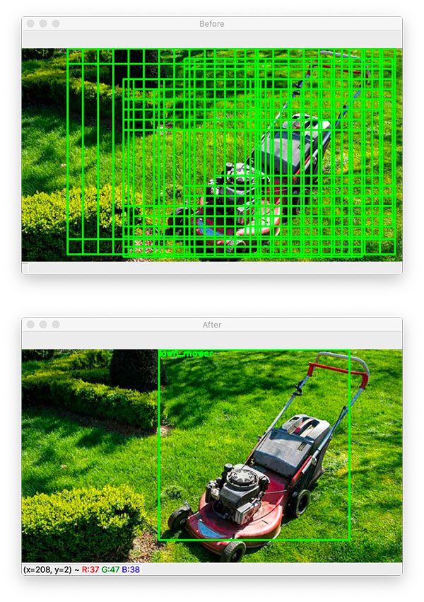
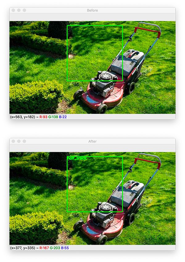
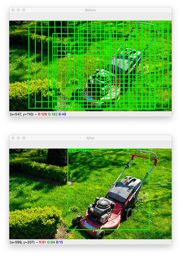
TensorFlow’s Object Detection API (TFOD API) is a library that we typically know for developing object detection models. We also need it to optimize models for the Nano’s GPU.

TensorFlow’s tf_trt_models is a wrapper around the TFOD API, which allows for building frozen graphs, a necessary for model deployment. More information on tf_trt_models can be found in this NVIDIA repository.

Again, ensure that all actions take place “in” your py3cv4 virtual environment:

$ cd ~
$ workon py3cv4

First, clone the models repository from TensorFlow:

$ git clone https://github.com/tensorflow/models

In order to be reproducible, you should checkout the following commit that supports TensorFlow 1.13.1:

$ cd models && git checkout -q b00783d

From there, install the COCO API for working with the COCO dataset and, in particular, object detection:

$ cd ~
$ git clone https://github.com/cocodataset/cocoapi.git
$ cd cocoapi/PythonAPI
$ python setup.py install

The next step is to compile the Protobuf libraries used by the TFOD API. The Protobuf libraries enable us (and therefore the TFOD API) to serialize structured data in a language-agnostic way:

$ cd ~/models/research/
$ protoc object_detection/protos/*.proto --python_out=.

From there, let’s configure a useful script I call setup.sh. This script will be needed each time you use the TFOD API for deployment on your Nano. Create such a file with the Nano editor:

$ nano ~/setup.sh

Insert the following lines in the new file:

#!/bin/sh

export PYTHONPATH=$PYTHONPATH:/home/`whoami`/models/research:\
/home/`whoami`/models/research/slim

The shebang at the top indicates that this file is executable and then the script configures your PYTHONPATH according to the TFOD API installation directory. Save and exit the file using the keyboard shortcuts shown at the bottom of the nano editor.

Step #13: Install NVIDIA’s ‘tf_trt_models’ for Jetson Nano

In this step, we’ll install the tf_trt_models library from GitHub. This package contains TensorRT-optimized models for the Jetson Nano.

First, ensure you’re working in the py3cv4 virtual environment:

$ workon py3cv4

Go ahead and clone the GitHub repo, and execute the installation script:

$ cd ~
$ git clone --recursive https://github.com/NVIDIA-Jetson/tf_trt_models.git
$ cd tf_trt_models
$ ./install.sh

That’s all there is to it. In the next step, we’ll install OpenCV!

Step #14: Install OpenCV 4.1.2 on Jetson Nano

In this section, we will install the OpenCV library with CUDA support on our Jetson Nano.

OpenCV is the common library we use for image processing, deep learning via the DNN module, and basic display tasks. I’ve created an OpenCV Tutorial for you if you’re interested in learning some of the basics.

CUDA is NVIDIA’s set of libraries for working with their GPUs. Some non-deep learning tasks can actually run on a CUDA-capable GPU faster than on a CPU. Therefore, we’ll install OpenCV with CUDA support, since the NVIDIA Jetson Nano has a small CUDA-capable GPU.

This section of the tutorial is based on the hard work of the owners of the PythOps website.

We will be compiling from source, so first let’s download the OpenCV source code from GitHub:

$ cd ~
$ wget -O opencv.zip https://github.com/opencv/opencv/archive/4.1.2.zip
$ wget -O opencv_contrib.zip https://github.com/opencv/opencv_contrib/archive/4.1.2.zip

Notice that the versions of OpenCV and OpenCV-contrib match. The versions must match for compatibility.

From there, extract the files and rename the directories for convenience:

$ unzip opencv.zip
$ unzip opencv_contrib.zip
$ mv opencv-4.1.2 opencv
$ mv opencv_contrib-4.1.2 opencv_contrib

Go ahead and activate your Python virtual environment if it isn’t already active:

$ workon py3cv4

And change into the OpenCV directory, followed by creating and entering a build directory:

$ cd opencv
$ mkdir build
$ cd build

It is very important that you enter the next CMake command while you are inside (1) the ~/opencv/build directory and (2) the py3cv4 virtual environment. Take a second now to verify:

(py3cv4) $ pwd
/home/nvidia/opencv/build

I typically don’t show the name of the virtual environment in the bash prompt because it takes up space, but notice how I have shown it at the beginning of the prompt above to indicate that we are “in” the virtual environment.

Additionally, the result of the pwd command indicates we are “in” the build/ directory.

Provided you’ve met both requirements, you’re now ready to use the CMake compile prep tool:

$ cmake -D CMAKE_BUILD_TYPE=RELEASE \
	-D WITH_CUDA=ON \
	-D CUDA_ARCH_PTX="" \
	-D CUDA_ARCH_BIN="5.3,6.2,7.2" \
	-D WITH_CUBLAS=ON \
	-D WITH_LIBV4L=ON \
	-D BUILD_opencv_python3=ON \
	-D BUILD_opencv_python2=OFF \
	-D BUILD_opencv_java=OFF \
	-D WITH_GSTREAMER=ON \
	-D WITH_GTK=ON \
	-D BUILD_TESTS=OFF \
	-D BUILD_PERF_TESTS=OFF \
	-D BUILD_EXAMPLES=OFF \
	-D OPENCV_ENABLE_NONFREE=ON \
	-D OPENCV_EXTRA_MODULES_PATH=/home/`whoami`/opencv_contrib/modules ..

There are a lot of compiler flags here, so let’s review them. Notice that WITH_CUDA=ON is set, indicating that we will be compiling with CUDA optimizations.

Secondly, notice that we have provided the path to our opencv_contrib folder in the OPENCV_EXTRA_MODULES_PATH, and we have set OPENCV_ENABLE_NONFREE=ON, indicating that we are installing the OpenCV library with full support for external and patented algorithms.

Be sure to copy the entire command above, including the .. at the very bottom. When CMake finishes, you’ll encounter the following output in your terminal:

Figure 10: It is critical to inspect your CMake output when installing the OpenCV computer vision library on an NVIDIA Jetson Nano prior to kicking off the compile process.

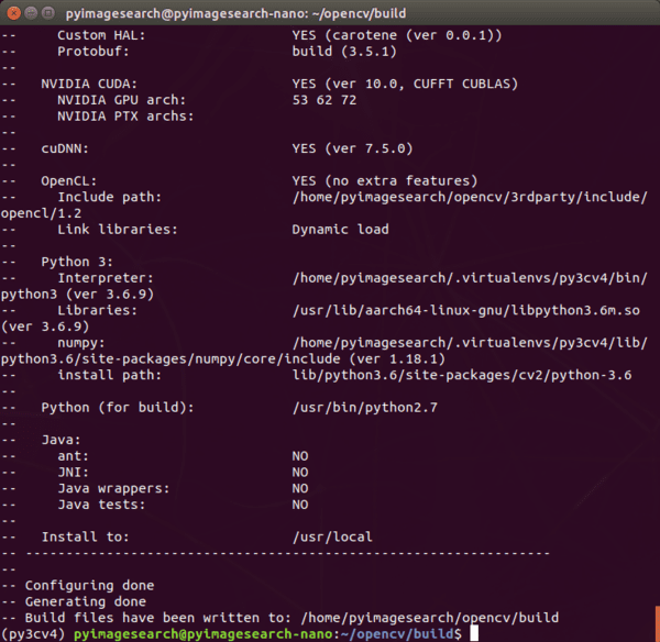
I highly recommend you scroll up and read the terminal output with a keen eye to see if there are any errors. Errors need to be resolved before moving on. If you do encounter an error, it is likely that one or more prerequisites from Steps #5-#11 are not installed properly. Try to determine the issue, and fix it.

If you do fix an issue, then you’ll need to delete and re-creating your build directory before running CMake again:

$ cd ..
$ rm -rf build
$ mkdir build
$ cd build
# run CMake command again

When you’re satisfied with your CMake output, it is time to kick of the compilation process with Make:

$ make -j4

Compiling OpenCV will take approximately 2.5 hours. When it is done, you’ll see 100%, and your bash prompt will return:

Figure 11: Once your 
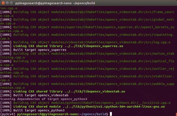
make command reaches 100% you can proceed with setting up your NVIDIA Jetson Nano for computer vision and deep learning.

From there, we need to finish the installation. First, run the install command:

$ sudo make install

Then, we need to create a symbolic link from OpenCV’s installation directory to the virtual environment. A symbolic link is like a pointer in that a special operating system file points from one place to another on your computer (in this case our Nano). Let’s create the sym-link now:

$ cd ~/.virtualenvs/py3cv4/lib/python3.6/site-packages/
$ ln -s /home/`whoami`/opencv-4.1.2/build/lib/python3/cv2.cpython-36m-aarch64-linux-gnu.so cv2.so

OpenCV is officially installed. In the next section, we’ll install a handful of useful libraries to accompany everything we’ve installed so far.

Step #15: Install other useful libraries via pip

In this section, we’ll use pip to install additional packages into our virtual environment.

Go ahead and activate your virtual environment:

$ workon py3cv4

And then install the following packages for machine learning, image processing, and plotting:

$ pip install matplotlib scikit-learn
$ pip install pillow imutils scikit-image

Followed by Davis King’s dlib library:

$ pip install dlib

Note: While you may be tempted to compile dlib with CUDA capability for your NVIDIA Jetson Nano, currently dlib does not support the Nano’s GPU. Sources: (1) dlib GitHub issues and (2) NVIDIA devtalk forums.

Now go ahead and install Flask, a Python micro web server; and Jupyter, a web-based Python environment:

$ pip install flask jupyter

And finally, install our XML tool for the TFOD API, and progressbar for keeping track of terminal programs that take a long time:

$ pip install lxml progressbar2

Great job, but the party isn’t over yet. In the next step, we’ll test our installation.

Step #16: Testing and Validation

I always like to test my installation at this point to ensure that everything is working as I expect. This quick verification can save time down the road when you’re ready to deploy computer vision and deep learning projects on your NVIDIA Jetson Nano.

Testing TensorFlow and Keras

To test TensorFlow and Keras, simply import them in a Python shell:

$ workon py3cv4
$ python
>>> import tensorflow
>>> import keras
>>> print(tensorflow.__version__)
1.13.1
>>> print(keras.__version__)
2.3.0

Again, we are purposely not using TensorFlow 2.0. As of March 2020, when this post was written, TensorFlow 2.0 is/was not supported by TensorRT and it has memory leak issues.

Testing TFOD API and TRT Models

To test the TFOD API, we first need to run the setup script:

$ cd ~
$ ./setup.sh

And then execute the test routine as shown in Figure 12:

Figure 12: Ensure that your NVIDIA Jetson Nano passes all TensorFlow Object Detection (TFOD) API tests before moving on with your embedded computer vision and deep learning install.

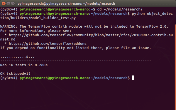
Assuming you see “OK” next to each test that was run, you are good to go.
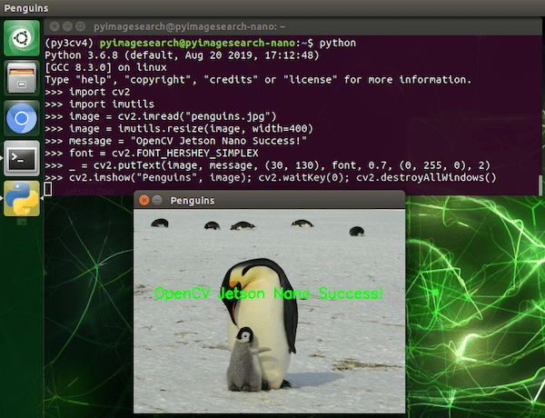
Testing OpenCV

To test OpenCV, we’ll simply import it in a Python shell and load + display an image:

$ workon py3cv4
$ wget -O penguins.jpg http://pyimg.co/avp96
$ python
>>> import cv2
>>> import imutils
>>> image = cv2.imread("penguins.jpg")
>>> image = imutils.resize(image, width=400)
>>> message = "OpenCV Jetson Nano Success!"
>>> font = cv2.FONT_HERSHEY_SIMPLEX
>>> _ = cv2.putText(image, message, (30, 130), font, 0.7, (0, 255, 0), 2)
>>> cv2.imshow("Penguins", image); cv2.waitKey(0); cv2.destroyAllWindows()
Figure 13: OpenCV (compiled with CUDA) for computer vision with Python is working on our NVIDIA Jetson Nano.

Testing your webcam

In this section, we’ll develop a quick and dirty script to test your NVIDIA Jetson Nano camera using either (1) a PiCamera or (2) a USB camera.

Did you know that the NVIDIA Jetson Nano is compatible with your Raspberry Pi picamera?

In fact it is, but it requires a long source string to interact with the driver. In this section, we’ll fire up a script to see how it works.

First, connect your PiCamera to your Jetson Nano with the ribbon cable as shown:

Figure 14: Your NVIDIA Jetson Nano is compatible with your Raspberry Pi’s PiCamera connected to the MIPI port.

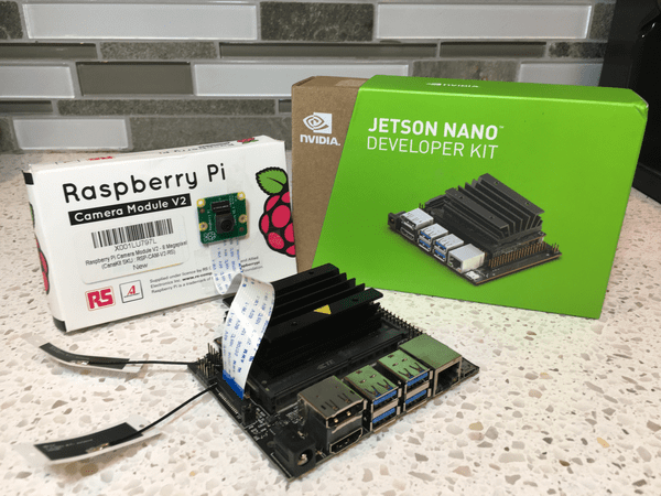
Next, be sure to grab the “Downloads” associated with this blog post for the test script. Let’s review the test_camera_nano.py script now:

# import the necessary packages
from imutils.video import VideoStream
import imutils
import time
import cv2

# grab a reference to the webcam
print("[INFO] starting video stream...")
#vs = VideoStream(src=0).start()
vs = VideoStream(src="nvarguscamerasrc ! video/x-raw(memory:NVMM), " \
	"width=(int)1920, height=(int)1080,format=(string)NV12, " \
	"framerate=(fraction)30/1 ! nvvidconv ! video/x-raw, " \
	"format=(string)BGRx ! videoconvert ! video/x-raw, " \
	"format=(string)BGR ! appsink").start()
time.sleep(2.0)

This script uses both OpenCV and imutils as shown in the imports on Lines 2-4.

Using the video module of imutils, let’s create a VideoStream on Lines 9-14:

  • USB Camera: Currently commented out on Line 9, to use your USB webcam, you simply need to provide src=0 or another device ordinal if you have more than one USB camera connected to your Nano
  • PiCamera: Currently active on Lines 10-14, a lengthy src string is used to work with the driver on the Nano to access a PiCamera plugged into the MIPI port. As you can see, the width and height in the format string indicate 1080p resolution. You can also use other resolutions that your PiCamera is compatible with

We’re more interested in the PiCamera right now, so let’s focus on Lines 10-14. These lines activate a stream for the Nano to use the PiCamera interface. Take note of the commas, exclamation points, and spaces. You definitely want to get the src string correct, so enter all parameters carefully!

Next, we’ll capture and display frames:

# loop over frames
while True:
	# grab the next frame
	frame = vs.read()

	# resize the frame to have a maximum width of 500 pixels
	frame = imutils.resize(frame, width=500)

	# show the output frame
	cv2.imshow("Frame", frame)
	key = cv2.waitKey(1) & 0xFF

	# if the `q` key was pressed, break from the loop
	if key == ord("q"):
		break

# release the video stream and close open windows
vs.stop()
cv2.destroyAllWindows()

Here we begin looping over frames. We resize the frame, and display it to our screen in an OpenCV window. If the q key is pressed, we exit the loop and cleanup.

To execute the script, simply enter the following command:

$ workon py3cv4
$ python test_camera_nano.py
Figure 15: Testing a PiCamera with the NVIDIA Jetson Nano configured for computer vision and deep learning.

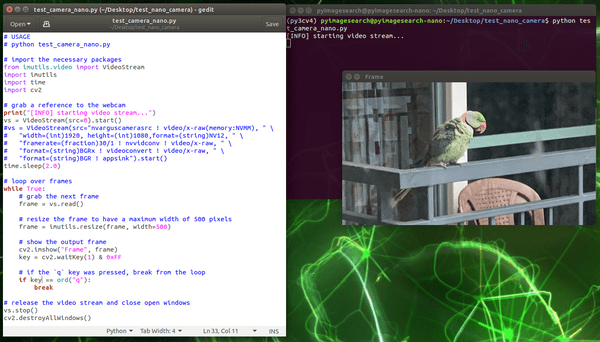
As you can see, now our PiCamera is working properly with the NVIDIA Jetson Nano.

Is there a faster way to get up and running?

Figure 16: Pick up your copy of Raspberry Pi for Computer Vision to gain access to the book, code, and three pre-configured .imgs: (1) NVIDIA Jetson Nano, (2) Raspberry Pi 3B+ / 4B, and (3) Raspberry Pi Zero W. This book will help you get your start in edge, IoT, and embedded computer vision and deep learning.

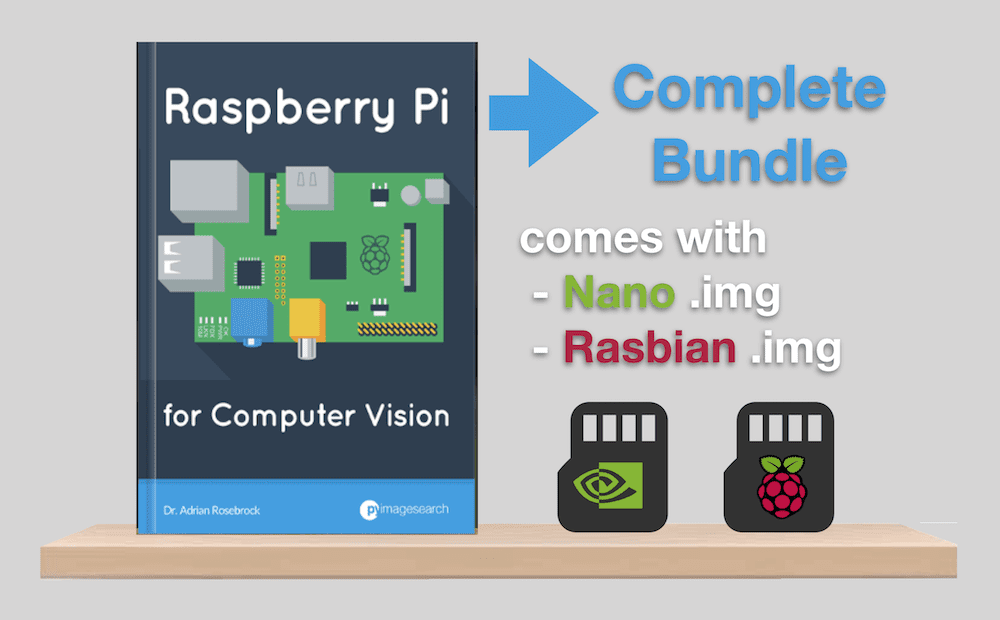
As an alternative to the painful, tedious, and time consuming process of configuring your Nano over the course of 2+ days, I suggest grabbing a copy off the Complete Bundle of Raspberry Pi for Computer Vision.

My book includes a pre-configured Nano .img developed with my team that is ready to go out of the box. It includes TensorFlow/Keras, TensorRT, OpenCV, scikit-image, scikit-learn, and more.

All you need to do is simply:

  1. Download the Jetson Nano .img file
  2. Flash it to your microSD card
  3. Boot your Nano
  4. And begin your projects

The .img file is worth the price of the Complete Bundle bundle alone.

As Peter Lans, a Senior Software Consultant, said:

Setting up a development environment for the Jetson Nano is horrible to do. After a few attempts, I gave up and left it for another day.

Until now my Jetson does what it does best: collecting dust in a drawer. But now I have an excuse to clean it and get it running again.

Besides the fact that Adrian’s material is awesome and comprehensive, the pre-configured Nano .img bonus is the cherry on the pie, making the price of Raspberry Pi for Computer Vision even more attractive.

To anyone interested in Adrian’s RPi4CV book, be fair to yourself and calculate the hours you waste getting nowhere. It will make you realize that you’ll have spent more in wasted time than on the book bundle.

One of my Twitter followers echoed the statement:

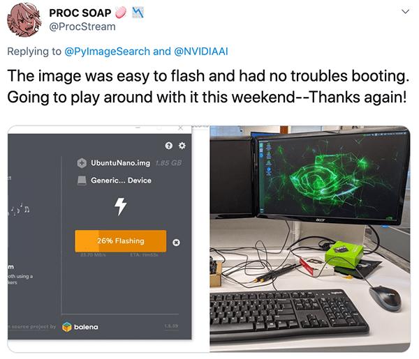
My .img files are updated on a regular basis and distributed to customers. I also provide priority support to customers of my books and courses, something that I’m unable to offer for free to everyone on the internet who visits this website.

Simply put, if you need support with your Jetson Nano from me, I recommend picking up a copy of Raspberry Pi for Computer Vision, which offers the best embedded computer vision and deep learning education available on the internet.

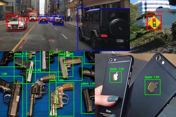
In addition to the .img files, RPi4CV covers how to successfully apply Computer Vision, Deep Learning, and OpenCV to embedded devices such as the:

  • Raspberry Pi
  • Intel Movidus NCS
  • Google Coral
  • NVIDIA Jetson Nano

Inside, you’ll find over 40 projects (including 60+ chapters) on embedded Computer Vision and Deep Learning.

A handful of the highlighted projects include:

  • Traffic counting and vehicle speed detection
  • Real-time face recognition
  • Building a classroom attendance system
  • Automatic hand gesture recognition
  • Daytime and nighttime wildlife monitoring
  • Security applications
  • Deep Learning classificationobject detection, and human pose estimation on resource-constrained devices
  • … and much more!

If you’re just as excited as I am, grab the free table of contents by clicking here:

Summary

In this tutorial, we configured our NVIDIA Jetson Nano for Python-based deep learning and computer vision.

We began by flashing the NVIDIA Jetpack .img. From there we installed prerequisites. We then configured a Python virtual environment for deploying computer vision and deep learning projects.

Inside our virtual environment, we installed TensorFlow, TensorFlow Object Detection (TFOD) API, TensorRT, and OpenCV.

We wrapped up by testing our software installations. We also developed a quick Python script to test both PiCamera and USB cameras.

If you’re interested in a computer vision and deep learning on the Raspberry Pi and NVIDIA Jetson Nano, be sure to pick up a copy of Raspberry Pi for Computer Vision.

To download the source code to this post (and be notified when future tutorials are published here on PyImageSearch), just enter your email address in the form below!

Download the Source Code and FREE 17-page Resource Guide

Enter your email address below to get a .zip of the code and a FREE 17-page Resource Guide on Computer Vision, OpenCV, and Deep Learning. Inside you’ll find my hand-picked tutorials, books, courses, and libraries to help you master CV and DL!

The post How to configure your NVIDIA Jetson Nano for Computer Vision and Deep Learning appeared first on PyImageSearch.


Autoencoders for Content-based Image Retrieval with Keras and TensorFlow

$
0
0

In this tutorial, you will learn how to use convolutional autoencoders to create a Content-based Image Retrieval system (i.e., image search engine) using Keras and TensorFlow.

A few weeks ago, I authored a series of tutorials on autoencoders:

  1. Part 1: Intro to autoencoders
  2. Part 2: Denoising autoencoders
  3. Part 3: Anomaly detection with autoencoders

The tutorials were a big hit; however, one topic I did not touch on was Content-based Image Retrieval (CBIR), which is really just a fancy academic word for image search engines.

Image search engines are similar to text search engines, only instead of presenting the search engine with a text query, you instead provide an image querythe image search engine then finds all visually similar/relevant images in its database and returns them to you (just as a text search engine would return links to articles, blog posts, etc.).

Deep learning-based CBIR and image retrieval can be framed as a form of unsupervised learning:

  • When training the autoencoder, we do not use any class labels
  • The autoencoder is then used to compute the latent-space vector representation for each image in our dataset (i.e., our “feature vector” for a given image)
  • Then, at search time, we compute the distance between the latent-space vectors — the smaller the distance, the more relevant/visually similar two images are

We can thus break up the CBIR project into three distinct phases:

  1. Phase #1: Train the autoencoder
  2. Phase #2: Extract features from all images in our dataset by computing their latent-space representations using the autoencoder
  3. Phase #3: Compare latent-space vectors to find all relevant images in the dataset

I’ll show you how to implement each of these phases in this tutorial, leaving you with a fully functioning autoencoder and image retrieval system.

To learn how to use autoencoders for image retrieval with Keras and TensorFlow, just keep reading!

Looking for the source code to this post?

Jump Right To The Downloads Section

Autoencoders for Content-based Image Retrieval with Keras and TensorFlow

In the first part of this tutorial, we’ll discuss how autoencoders can be used for image retrieval and building image search engines.

From there, we’ll implement a convolutional autoencoder that we’ll then train on our image dataset.

Once the autoencoder is trained, we’ll compute feature vectors for each image in our dataset. Computing the feature vector for a given image requires only a forward-pass of the image through the network — the output of the encoder (i.e., the latent-space representation) will serve as our feature vector.

After all images are encoded, we can then compare vectors by computing the distance between them. Images with a smaller distance will be more similar than images with a larger distance.

Finally, we will review the results of applying our autoencoder for image retrieval.

How can autoencoders be used for image retrieval and image search engines?

The process of using an autoencoder for an image search engine using Keras and TensorFlow. Top: We train an autoencoder on our input dataset in an unsupervised fashion. Bottom: We use the autoencoder to extract and store features in an index and then search the index with a query image's feature vector, finding the most similar images via a distance metric.
Figure 1: The process of using an autoencoder for an image search engine using Keras and TensorFlow. Top: We train an autoencoder on our input dataset in an unsupervised fashion. Bottom: We use the autoencoder to extract and store features in an index and then search the index with a query image’s feature vector, finding the most similar images via a distance metric.

As discussed in my intro to autoencoders tutorial, autoencoders:

  1. Accept an input set of data (i.e., the input)
  2. Internally compress the input data into a latent-space representation (i.e., a single vector that compresses and quantifies the input)
  3. Reconstruct the input data from this latent representation (i.e., the output)

To build an image retrieval system with an autoencoder, what we really care about is that latent-space representation vector.

Once an autoencoder has been trained to encode images, we can:

  1. Use the encoder portion of the network to compute the latent-space representation of each image in our dataset — this representation serves as our feature vector that quantifies the contents of an image
  2. Compare the feature vector from our query image to all feature vectors in our dataset (typically you would use either the Euclidean or cosine distance)

Feature vectors that have a smaller distance will be considered more similar, while images with a larger distance will be deemed less similar.

We can then sort our results based on the distance (from smallest to largest) and finally display the image retrieval results to the end user.

Project structure

Go ahead and grab this tutorial’s files from the “Downloads” section. From there, extract the .zip, and open the folder for inspection:

$ tree --dirsfirst
.
├── output
│   ├── autoencoder.h5
│   ├── index.pickle
│   ├── plot.png
│   └── recon_vis.png
├── pyimagesearch
│   ├── __init__.py
│   └── convautoencoder.py
├── index_images.py
├── search.py
└── train_autoencoder.py

2 directories, 9 files

This tutorial consists of three Python driver scripts:

  • train_autoencoder.py: Trains an autoencoder on the MNIST handwritten digits dataset using the ConvAutoencoder CNN/class
  • index_images.py: Using the encoder portion of our trained autoencoder, we’ll compute feature vectors for each image in the dataset and add the features to a searchable index
  • search.py: Queries our index for similar images using a similarity metric

Our output/ directory contains our trained autoencoder and index. Training also results in a training history plot and visualization image that can be exported to the output/ folder.

Implementing our convolutional autoencoder architecture for image retrieval

Before we can train our autoencoder, we must first implement the architecture itself. To do so, we’ll be using Keras and TensorFlow.

We’ve already implemented convolutional autoencoders a handful of times before on the PyImageSearch blog, so while I’ll be covering the complete implementation here today, you’ll want to refer to my intro to autoencoders tutorial for more details.

Open up the convautoencoder.py file in the pyimagesearch module, and let’s get to work:

# import the necessary packages
from tensorflow.keras.layers import BatchNormalization
from tensorflow.keras.layers import Conv2D
from tensorflow.keras.layers import Conv2DTranspose
from tensorflow.keras.layers import LeakyReLU
from tensorflow.keras.layers import Activation
from tensorflow.keras.layers import Flatten
from tensorflow.keras.layers import Dense
from tensorflow.keras.layers import Reshape
from tensorflow.keras.layers import Input
from tensorflow.keras.models import Model
from tensorflow.keras import backend as K
import numpy as np

Imports include a selection from tf.keras as well as NumPy. We’ll go ahead and define our autoencoder class next:

class ConvAutoencoder:
	@staticmethod
	def build(width, height, depth, filters=(32, 64), latentDim=16):
		# initialize the input shape to be "channels last" along with
		# the channels dimension itself
		# channels dimension itself
		inputShape = (height, width, depth)
		chanDim = -1

		# define the input to the encoder
		inputs = Input(shape=inputShape)
		x = inputs

		# loop over the number of filters
		for f in filters:
			# apply a CONV => RELU => BN operation
			x = Conv2D(f, (3, 3), strides=2, padding="same")(x)
			x = LeakyReLU(alpha=0.2)(x)
			x = BatchNormalization(axis=chanDim)(x)

		# flatten the network and then construct our latent vector
		volumeSize = K.int_shape(x)
		x = Flatten()(x)
		latent = Dense(latentDim, name="encoded")(x)

Our ConvAutoencoder class contains one static method, build, which accepts five parameters: (1) width, (2) height, (3) depth, (4) filters, and (5) latentDim.

The Input is then defined for the encoder, at which point we use Keras’ functional API to loop over our filters and add our sets of CONV => LeakyReLU => BN layers (Lines 21-33).

We then flatten the network and construct our latent vector (Lines 36-38).

The latent-space representation is the compressed form of our data — once trained, the output of this layer will be our feature vector used to quantify and represent the contents of the input image.

From here, we will construct the input to the decoder portion of the network:

		# start building the decoder model which will accept the
		# output of the encoder as its inputs
		x = Dense(np.prod(volumeSize[1:]))(latent)
		x = Reshape((volumeSize[1], volumeSize[2], volumeSize[3]))(x)

		# loop over our number of filters again, but this time in
		# reverse order
		for f in filters[::-1]:
			# apply a CONV_TRANSPOSE => RELU => BN operation
			x = Conv2DTranspose(f, (3, 3), strides=2,
				padding="same")(x)
			x = LeakyReLU(alpha=0.2)(x)
			x = BatchNormalization(axis=chanDim)(x)

		# apply a single CONV_TRANSPOSE layer used to recover the
		# original depth of the image
		x = Conv2DTranspose(depth, (3, 3), padding="same")(x)
		outputs = Activation("sigmoid", name="decoded")(x)

		# construct our autoencoder model
		autoencoder = Model(inputs, outputs, name="autoencoder")

		# return the autoencoder model
		return autoencoder

The decoder model accepts the output of the encoder as its inputs (Lines 42 and 43).

Looping over filters in reverse order, we construct CONV_TRANSPOSE => LeakyReLU => BN layer blocks (Lines 47-52).

Lines 56-63 recover the original depth of the image.

We wrap up by constructing and returning our autoencoder model (Lines 60-63).

For more details on our implementation, be sure to refer to our intro to autoencoders with Keras and TensorFlow tutorial.

Creating the autoencoder training script using Keras and TensorFlow

With our autoencoder implemented, let’s move on to the training script (Phase #1).

Open the train_autoencoder.py script, and insert the following code:

# set the matplotlib backend so figures can be saved in the background
import matplotlib
matplotlib.use("Agg")

# import the necessary packages
from pyimagesearch.convautoencoder import ConvAutoencoder
from tensorflow.keras.optimizers import Adam
from tensorflow.keras.datasets import mnist
import matplotlib.pyplot as plt
import numpy as np
import argparse
import cv2

On Lines 2-12, we handle our imports. We’ll use the "Agg" backend of matplotlib so that we can export our training plot to disk. We need our custom ConvAutoencoder architecture class from the previous section. We will take advantage of the Adam optimizer as we train on the MNIST benchmarking dataset.

For visualization, we’ll employ OpenCV in the visualize_predictions helper function:

def visualize_predictions(decoded, gt, samples=10):
	# initialize our list of output images
	outputs = None

	# loop over our number of output samples
	for i in range(0, samples):
		# grab the original image and reconstructed image
		original = (gt[i] * 255).astype("uint8")
		recon = (decoded[i] * 255).astype("uint8")

		# stack the original and reconstructed image side-by-side
		output = np.hstack([original, recon])

		# if the outputs array is empty, initialize it as the current
		# side-by-side image display
		if outputs is None:
			outputs = output

		# otherwise, vertically stack the outputs
		else:
			outputs = np.vstack([outputs, output])

	# return the output images
	return outputs

Inside the visualize_predictions helper, we compare our original ground-truth input images (gt) to the output reconstructed images from the autoencoder (decoded) and generate a side-by-side comparison montage.

Line 16 initializes our list of output images.

We then loop over the samples:

  • Grabbing both the original and reconstructed images (Lines 21 and 22)
  • Stacking the pair of images side-by-side (Line 25)
  • Stacking the pairs vertically (Lines 29-34)

Finally, we return the visualization image to the caller (Line 37).

We’ll need a few command line arguments for our script to run from our terminal/command line:

# construct the argument parse and parse the arguments
ap = argparse.ArgumentParser()
ap.add_argument("-m", "--model", type=str, required=True,
	help="path to output trained autoencoder")
ap.add_argument("-v", "--vis", type=str, default="recon_vis.png",
	help="path to output reconstruction visualization file")
ap.add_argument("-p", "--plot", type=str, default="plot.png",
	help="path to output plot file")
args = vars(ap.parse_args())

Here we parse three command line arguments:

  • --model: Points to the path of our trained output autoencoder — the result of executing this script
  • --vis: The path to the output visualization image. We’ll name our visualization recon_vis.png by default
  • --plot: The path to our matplotlib output plot. A default of plot.png is assigned if this argument is not provided in the terminal

Now that our imports, helper function, and command line arguments are ready, we’ll prepare to train our autoencoder:

# initialize the number of epochs to train for, initial learning rate,
# and batch size
EPOCHS = 20
INIT_LR = 1e-3
BS = 32

# load the MNIST dataset
print("[INFO] loading MNIST dataset...")
((trainX, _), (testX, _)) = mnist.load_data()

# add a channel dimension to every image in the dataset, then scale
# the pixel intensities to the range [0, 1]
trainX = np.expand_dims(trainX, axis=-1)
testX = np.expand_dims(testX, axis=-1)
trainX = trainX.astype("float32") / 255.0
testX = testX.astype("float32") / 255.0

# construct our convolutional autoencoder
print("[INFO] building autoencoder...")
autoencoder = ConvAutoencoder.build(28, 28, 1)
opt = Adam(lr=INIT_LR, decay=INIT_LR / EPOCHS)
autoencoder.compile(loss="mse", optimizer=opt)

# train the convolutional autoencoder
H = autoencoder.fit(
	trainX, trainX,
	validation_data=(testX, testX),
	epochs=EPOCHS,
	batch_size=BS)

Hyperparameter constants including the number of training epochs, learning rate, and batch size are defined on Lines 51-53.

Our autoencoder (and therefore our CBIR system) will be trained on the MNIST handwritten digits dataset which we load from disk on Line 57.

To preprocess MNIST images, we add a channel dimension to the training/testing sets (Lines 61 and 62) and scale pixel intensities to the range [0, 1] (Lines 63 and 64).

With our data ready to go, Lines 68-70 compile our autoencoder with the Adam optimizer and mean-squared error loss.

Lines 73-77 then fit our model to the data (i.e., train our autoencoder).

Once the model is trained, we’ll make predictions with it:

# use the convolutional autoencoder to make predictions on the
# testing images, construct the visualization, and then save it
# to disk
print("[INFO] making predictions...")
decoded = autoencoder.predict(testX)
vis = visualize_predictions(decoded, testX)
cv2.imwrite(args["vis"], vis)

# construct a plot that plots and saves the training history
N = np.arange(0, EPOCHS)
plt.style.use("ggplot")
plt.figure()
plt.plot(N, H.history["loss"], label="train_loss")
plt.plot(N, H.history["val_loss"], label="val_loss")
plt.title("Training Loss and Accuracy")
plt.xlabel("Epoch #")
plt.ylabel("Loss/Accuracy")
plt.legend(loc="lower left")
plt.savefig(args["plot"])

# serialize the autoencoder model to disk
print("[INFO] saving autoencoder...")
autoencoder.save(args["model"], save_format="h5")

Lines 83 and 84 make predictions on the testing set and generate our autoencoder visualization using our helper function. Line 85 writes the visualization to disk using OpenCV.

Finally, we plot training history (Lines 88-97) and serialize our autoencoder to disk (Line 101).

In the next section, we’ll put the training script to work.

Training the autoencoder

We are now ready to train our convolutional autoencoder for image retrieval.

Make sure you use the “Downloads” section of this tutorial to download the source code, and from there, execute the following command to start the training process:

$ python train_autoencoder.py --model output/autoencoder.h5 \
    --vis output/recon_vis.png --plot output/plot.png
[INFO] loading MNIST dataset...
[INFO] building autoencoder...
Train on 60000 samples, validate on 10000 samples
Epoch 1/20
60000/60000 [==============================] - 73s 1ms/sample - loss: 0.0182 - val_loss: 0.0124
Epoch 2/20
60000/60000 [==============================] - 73s 1ms/sample - loss: 0.0101 - val_loss: 0.0092
Epoch 3/20
60000/60000 [==============================] - 73s 1ms/sample - loss: 0.0090 - val_loss: 0.0084
...
Epoch 18/20
60000/60000 [==============================] - 72s 1ms/sample - loss: 0.0065 - val_loss: 0.0067
Epoch 19/20
60000/60000 [==============================] - 73s 1ms/sample - loss: 0.0065 - val_loss: 0.0067
Epoch 20/20
60000/60000 [==============================] - 73s 1ms/sample - loss: 0.0064 - val_loss: 0.0067
[INFO] making predictions...
[INFO] saving autoencoder...

On my 3Ghz Intel Xeon W processor, the entire training process took ~24 minutes.

Looking at the plot in Figure 2, we can see that the training process was stable with no signs of overfitting:

Training an autoencoder with Keras and TensorFlow for Content-based Image Retrieval (CBIR).
Figure 2: Training an autoencoder with Keras and TensorFlow for Content-based Image Retrieval (CBIR).

Furthermore, the following reconstruction plot shows that our autoencoder is doing a fantastic job of reconstructing our input digits.

Figure 3: Visualizing reconstructed data from an autoencoder trained on MNIST using TensorFlow and Keras for image search engine purposes.

The fact that our autoencoder is doing such a good job also implies that our latent-space representation vectors are doing a good job compressing, quantifying, and representing the input image — having such a representation is a requirement when building an image retrieval system.

If the feature vectors cannot capture and quantify the contents of the image, then there is no way that the CBIR system will be able to return relevant images.

If you find that your autoencoder is failing to properly reconstruct your images, then it’s unlikely your autoencoder will perform well for image retrieval.

Take the proper care to train an accurate autoencoder — doing so will help ensure your image retrieval system returns similar images.

Implementing image indexer using the trained autoencoder

With our autoencoder successfully trained (Phase #1), we can move on to the feature extraction/indexing phase of the image retrieval pipeline (Phase #2).

This phase, at a bare minimum, requires us to use our trained autoencoder (specifically the “encoder” portion) to accept an input image, perform a forward pass, and then take the output of the encoder portion of the network to generate our index of feature vectors. These feature vectors are meant to quantify the contents of each image.

Optionally, we may also use specialized data structures such as VP-Trees and Random Projection Trees to improve the query speed of our image retrieval system.

Open up the index_images.py file in your directory structure and we’ll get started:

# import the necessary packages
from tensorflow.keras.models import Model
from tensorflow.keras.models import load_model
from tensorflow.keras.datasets import mnist
import numpy as np
import argparse
import pickle

# construct the argument parse and parse the arguments
ap = argparse.ArgumentParser()
ap.add_argument("-m", "--model", type=str, required=True,
	help="path to trained autoencoder")
ap.add_argument("-i", "--index", type=str, required=True,
	help="path to output features index file")
args = vars(ap.parse_args())

We begin with imports. Our tf.keras imports include (1) Model so we can construct our encoder, (2) load_model so we can load our autoencoder model we trained in the previous step, and (3) our mnist dataset. Our feature vector index will be serialized as a Python pickle file.

We have two required command line arguments:

  • --model: The trained autoencoder input path from the previous step
  • --index: The path to the output features index file in .pickle format

From here, we’ll load and preprocess our MNIST digit data:

# load the MNIST dataset
print("[INFO] loading MNIST training split...")
((trainX, _), (testX, _)) = mnist.load_data()

# add a channel dimension to every image in the training split, then
# scale the pixel intensities to the range [0, 1]
trainX = np.expand_dims(trainX, axis=-1)
trainX = trainX.astype("float32") / 255.0

Notice that the preprocessing steps are identical to that of our training procedure.

We’ll then load our autoencoder:

# load our autoencoder from disk
print("[INFO] loading autoencoder model...")
autoencoder = load_model(args["model"])

# create the encoder model which consists of *just* the encoder
# portion of the autoencoder
encoder = Model(inputs=autoencoder.input,
	outputs=autoencoder.get_layer("encoded").output)

# quantify the contents of our input images using the encoder
print("[INFO] encoding images...")
features = encoder.predict(trainX)

Line 28 loads our autoencoder (trained in the previous step) from disk.

Then, using the autoencoder’s input, we create a Model while only accessing the encoder portion of the network (i.e., the latent-space feature vector) as the output (Lines 32 and 33).

We then pass the MNIST digit image data through the encoder to compute our feature vectors (features) on Line 37.

Finally, we construct a dictionary map of our feature data:

# construct a dictionary that maps the index of the MNIST training
# image to its corresponding latent-space representation
indexes = list(range(0, trainX.shape[0]))
data = {"indexes": indexes, "features": features}

# write the data dictionary to disk
print("[INFO] saving index...")
f = open(args["index"], "wb")
f.write(pickle.dumps(data))
f.close()

Line 42 builds a data dictionary consisting of two components:

  • indexes: Integer indices of each MNIST digit image in the dataset
  • features: The corresponding feature vector for each image in the dataset

To close out, Lines 46-48 serialize the data to disk in Python’s pickle format.

Indexing our image dataset for image retrieval

We are now ready to quantify our image dataset using the autoencoder, specifically using the latent-space output of the encoder portion of the network.

To quantify our image dataset using the trained autoencoder, make sure you use the “Downloads” section of this tutorial to download the source code and pre-trained model.

From there, open up a terminal and execute the following command:

$ python index_images.py --model output/autoencoder.h5 \
	--index output/index.pickle
[INFO] loading MNIST training split...
[INFO] loading autoencoder model...
[INFO] encoding images...
[INFO] saving index...

If you check the contents of your output directory, you should now see your index.pickle file:

$ ls output/*.pickle
output/index.pickle

Implementing the image search and retrieval script using Keras and TensorFlow

Our final script, our image searcher, puts all the pieces together and allows us to complete our autoencoder image retrieval project (Phase #3). Again, we’ll be using Keras and TensorFlow for this implementation.

Open up the search.py script, and insert the following contents:

# import the necessary packages
from tensorflow.keras.models import Model
from tensorflow.keras.models import load_model
from tensorflow.keras.datasets import mnist
from imutils import build_montages
import numpy as np
import argparse
import pickle
import cv2

As you can see, this script needs the same tf.keras imports as our indexer. Additionally, we’ll use my build_montages convenience script in my imutils package to display our autoencoder CBIR results.

Let’s define a function to compute the similarity between two feature vectors:

def euclidean(a, b):
	# compute and return the euclidean distance between two vectors
	return np.linalg.norm(a - b)

Here we’re the Euclidean distance to calculate the similarity between two feature vectors, a and b.

There are multiple ways to compute distances — the cosine distance can be a good alternative for many CBIR applications. I also cover other distance algorithms inside the PyImageSearch Gurus course.

Next, we’ll define our searching function:

def perform_search(queryFeatures, index, maxResults=64):
	# initialize our list of results
	results = []

	# loop over our index
	for i in range(0, len(index["features"])):
		# compute the euclidean distance between our query features
		# and the features for the current image in our index, then
		# update our results list with a 2-tuple consisting of the
		# computed distance and the index of the image
		d = euclidean(queryFeatures, index["features"][i])
		results.append((d, i))

	# sort the results and grab the top ones
	results = sorted(results)[:maxResults]

	# return the list of results
	return results

Our perform_search function is responsible for comparing all feature vectors for similarity and returning the results.

This function accepts both the queryFeatures, a feature vector for the query image, and the index of all features to search through.

Our results will contain the top maxResults (in our case 64 is the default but we will soon override it to 225).

Line 17 initializes our list of results, which Lines 20-20 then populate. Here, we loop over all entries in our index, computing the Euclidean distance between our queryFeatures and the current feature vector in the index.

When it comes to the distance:

  • The smaller the distance, the more similar the two images are
  • The larger the distance, the less similar they are

We sort and grab the top results such that images that are more similar to the query are at the front of the list via Line 29.

Finally, we return the the search results to the calling function (Line 32).

With both our distance metric and searching utility defined, we’re now ready to parse command line arguments:

# construct the argument parse and parse the arguments
ap = argparse.ArgumentParser()
ap.add_argument("-m", "--model", type=str, required=True,
	help="path to trained autoencoder")
ap.add_argument("-i", "--index", type=str, required=True,
	help="path to features index file")
ap.add_argument("-s", "--sample", type=int, default=10,
	help="# of testing queries to perform")
args = vars(ap.parse_args())

Our script accepts three command line arguments:

  • --model: The path to the trained autoencoder from the “Training the autoencoder” section
  • --index: Our index of features to search through (i.e., the serialized index from the “Indexing our image dataset for image retrieval” section)
  • --sample: The number of testing queries to perform with a default of 10

Now, let’s load and preprocess our digit data:

# load the MNIST dataset
print("[INFO] loading MNIST dataset...")
((trainX, _), (testX, _)) = mnist.load_data()

# add a channel dimension to every image in the dataset, then scale
# the pixel intensities to the range [0, 1]
trainX = np.expand_dims(trainX, axis=-1)
testX = np.expand_dims(testX, axis=-1)
trainX = trainX.astype("float32") / 255.0
testX = testX.astype("float32") / 255.0

And then we’ll load our autoencoder and index:

# load the autoencoder model and index from disk
print("[INFO] loading autoencoder and index...")
autoencoder = load_model(args["model"])
index = pickle.loads(open(args["index"], "rb").read())

# create the encoder model which consists of *just* the encoder
# portion of the autoencoder
encoder = Model(inputs=autoencoder.input,
	outputs=autoencoder.get_layer("encoded").output)

# quantify the contents of our input testing images using the encoder
print("[INFO] encoding testing images...")
features = encoder.predict(testX)

Here, Line 57 loads our trained autoencoder from disk, while Line 58 loads our pickled index from disk.

We then build a Model that will accept our images as an input and the output of our encoder layer (i.e., feature vector) as our model’s output (Lines 62 and 63).

Given our encoder, Line 67 performs a forward-pass of our set of testing images through the network, generating a list of features to quantify them.

We’ll now take a random sample of images, marking them as queries:

# randomly sample a set of testing query image indexes
queryIdxs = list(range(0, testX.shape[0]))
queryIdxs = np.random.choice(queryIdxs, size=args["sample"],
	replace=False)

# loop over the testing indexes
for i in queryIdxs:
	# take the features for the current image, find all similar
	# images in our dataset, and then initialize our list of result
	# images
	queryFeatures = features[i]
	results = perform_search(queryFeatures, index, maxResults=225)
	images = []

	# loop over the results
	for (d, j) in results:
		# grab the result image, convert it back to the range
		# [0, 255], and then update the images list
		image = (trainX[j] * 255).astype("uint8")
		image = np.dstack([image] * 3)
		images.append(image)

	# display the query image
	query = (testX[i] * 255).astype("uint8")
	cv2.imshow("Query", query)

	# build a montage from the results and display it
	montage = build_montages(images, (28, 28), (15, 15))[0]
	cv2.imshow("Results", montage)
	cv2.waitKey(0)

Lines 70-72 sample a set of testing image indices, marking them as our search engine queries.

We then loop over the queries beginning on Line 75. Inside, we:

  • Grab the queryFeatures, and perform the search (Lines 79 and 80)
  • Initialize a list to hold our result images (Line 81)
  • Loop over the results, scaling the image back to the range [0, 255], creating an RGB representation from the grayscale image for display, and then adding it to our images results (Lines 84-89)
  • Display the query image in its own OpenCV window (Lines 92 and 93)
  • Display a montage of search engine results (Lines 96 and 97)
  • When the user presses a key, we repeat the process (Line 98) with a different query image; you should continue to press a key as you inspect results until all of our query samples have been searched

To recap our search searching script, first we loaded our autoencoder and index.

We then grabbed the encoder portion of the autoencoder and used it to quantify our images (i.e., create feature vectors).

From there, we created a sample of random query images to test our searching method which is based on the Euclidean distance computation. Smaller distances indicate similar images — the similar images will be shown first because our results are sorted (Line 29).

We searched our index for each query showing only a maximum of maxResults in each montage.

In the next section, we’ll get the chance to visually validate how our autoencoder-based search engine works.

Image retrieval results using autoencoders, Keras, and TensorFlow

We are now ready to see our autoencoder image retrieval system in action!

Start by making sure you have:

  1. Used the “Downloads” section of this tutorial to download the source code
  2. Executed the train_autoencoder.py file to train the convolutional autoencoder
  3. Run the index_images.py to quantify each image in our dataset

From there, you can execute the search.py script to perform a search:

$ python search.py --model output/autoencoder.h5 \
	--index output/index.pickle
[INFO] loading MNIST dataset...
[INFO] loading autoencoder and index...
[INFO] encoding testing images...

Below is an example providing a query image containing the digit 9 (top) along with the search results from our autoencoder image retrieval system (bottom):

Figure 4: Top: MNIST query image. Bottom: Autoencoder-based image search engine results. We learn how to use Keras, TensorFlow, and OpenCV to build a Content-based Image Retrieval (CBIR) system.

Here, you can see that our system has returned search results also containing nines.

Let’s now use a 2 as our query image:

Figure 5: Content-based Image Retrieval (CBIR) is used with an autoencoder to find images of handwritten 2s in our dataset.

Sure enough, our CBIR system returns digits containing twos, implying that latent-space representation has correctly quantified what a 2 looks like.

Here’s an example of using a 4 as a query image:

Figure 6: Content-based Image Retrieval (CBIR) is used with an autoencoder to find images of handwritten 4s in our dataset.

Again, our autoencoder image retrieval system returns all fours as the search results.

Let’s look at one final example, this time using a 0 as a query image:

Figure 7: No image search engine is perfect. Here, there are mistakes in our results from searching MNIST for handwritten 0s using an autoencoder-based image search engine built with TensorFlow, Keras, and OpenCV.

This result is more interesting — note the two highlighted results in the screenshot.

The first highlighted result is likely a 5, but the tail of the five seems to be connecting to the middle part, creating a digit that looks like a cross between a 0 and an 8.

We then have what I think is an 8 near the bottom of the search results (also highlighted in red). Again, we can appreciate how our image retrieval system may see that 8 as visually similar to a 0.

Tips to improve autoencoder image retrieval accuracy and speed

In this tutorial, we performed image retrieval on the MNIST dataset to demonstrate how autoencoders can be used to build image search engines.

However, you will more than likely want to use your own image dataset rather than the MNIST dataset.

Swapping in your own dataset is as simple as replacing the MNIST dataset loader helper function with your own dataset loader — you can then train an autoencoder on your dataset.

However, make sure your autoencoder accuracy is sufficient.

If your autoencoder cannot reasonably reconstruct your input data, then:

  1. The autoencoder is failing to capture the patterns in your dataset
  2. The latent-space vector will not properly quantify your images
  3. And without proper quantification, your image retrieval system will return irrelevant results

Therefore, nearly the entire accuracy of your CBIR system hinges on your autoencoder — take the time to ensure it is properly trained.

Once your autoencoder is performing well, you can then move on to optimizing the speed of your search procedure.

Secondly, you should also consider the scalability of your CBIR system.

Our implementation here is an example of a linear search with O(N) complexity, meaning that it will not scale well.

To improve the speed of the retrieval system, you should use Approximate Nearest Neighbor algorithms and specialized data structures such as VP-Trees, Random Projection trees, etc., which can reduce the computational complexity to O(log N).

To learn more about these techniques, refer to my article on Building an Image Hashing Search Engine with VP-Trees and OpenCV.

What’s next?

Figure 8: In my computer vision course, I cover what most of us reading this article wish we had learned in undergraduate classes at our college/university. My course is practical, hands-on, and fun. You’ll also gain access to me, my team, and other students/graduates in the community forums. Join the course and discussion today!

If you want to increase your computer vision knowledge, then look no further than the PyImageSearch Gurus course and community.

Inside the course you’ll find:

  • An actionable, real-world course on OpenCV and computer vision. Each lesson in PyImageSearch Gurus is taught in the same trademark, hands-on, easy-to-understand PyImageSearch style that you know and love
  • The most comprehensive computer vision education online today. The PyImageSearch Gurus course covers 13 modules broken out into 168 lessons, with over 2,161 pages of content. You won’t find a more detailed computer vision course anywhere else online; I guarantee it
  • A community of like-minded developers, researchers, and students just like you, who are eager to learn computer vision and level-up their skills

The course covers breadth and depth in the following subject areas, giving you the skills to rise in the ranks at your institution or even to land that next job:

  • Automatic License Plate Recognition (ANPR) — recognize license plates of vehicles, or apply the concepts to your own OCR project
  • Face Detection and Recognition — recognize who’s entering/leaving your house, build a smart classroom attendance system, or identify who’s who in your collection of family portraits
  • Image Search Engines also known as Content Based Image Retrieval (CBIR)
  • Object Detection — and my 6-step framework to accomplish it
  • Big Data methodologies — use Hadoop for executing image processing algorithms in parallel on large computing clusters
  • Machine Learning and Deep Learning — learn just what you need to know to be dangerous in today’s AI age, and prime your pump for even more advanced deep learning inside my book, Deep Learning for Computer Vision with Python

If the course sounds interesting to you, I’d love to send you 10 free sample lessons and the entire course syllabus so you can get a feel for what the course has to offer. Just click the link below!

Master computer vision inside PyImageSearch Gurus!

Summary

In this tutorial, you learned how to use convolutional autoencoders for image retrieval using TensorFlow and Keras.

To create our image retrieval system, we:

  1. Trained a convolutional autoencoder on our image dataset
  2. Used the trained autoencoder to compute the latent-space representation of each image in our dataset — this representation serves as our feature vector that quantifies the contents of the image
  3. Compared the feature vector from our query image to all feature vectors in our dataset using a distance function (in this case, the Euclidean distance, but cosine distance would also work well here). The smaller the distance between the vectors the more similar our images were.

We then sorted our results based on the computed distance and displayed our results to the user.

Autoencoders can be extremely useful for CBIR applications — the downside is that they require a lot of training data, which you may or may not have.

More advanced deep learning image retrieval systems rely on siamese networks and triplet loss to embed vectors for images such that more similar images lie closer together in a Euclidean space, while less similar images are farther away — I’ll be covering these types of network architectures and techniques at a future date.

To download the source code to this post (including the pre-trained autoencoder), just enter your email address in the form below!

Download the Source Code and FREE 17-page Resource Guide

Enter your email address below to get a .zip of the code and a FREE 17-page Resource Guide on Computer Vision, OpenCV, and Deep Learning. Inside you’ll find my hand-picked tutorials, books, courses, and libraries to help you master CV and DL!

The post Autoencoders for Content-based Image Retrieval with Keras and TensorFlow appeared first on PyImageSearch.

Blur and anonymize faces with OpenCV and Python

$
0
0


In this tutorial, you will learn how to blur and anonymize faces using OpenCV and Python.

Today’s blog post is inspired by an email I received last week from PyImageSearch reader, Li Wei:

Hi Adrian, I’m working on a research project for my university.

I’m in charge of creating the dataset but my professor has asked me to “anonymize” each image by detecting faces and then blurring them to ensure privacy is protected and that no face can be recognized (apparently this is a requirement at my institution before we publicly distribute the dataset).

Do you have any tutorials on face anonymization? How can I blur faces using OpenCV?

Thanks,

Li Wei

Li asks a great question — we often utilize face detection in our projects, typically as the first step in a face recognition pipeline.

But what if we wanted to do the “opposite” of face recognition? What if we instead wanted to anonymize the face by blurring it, thereby making it impossible to identify the face?

Practical applications of face blurring and anonymization include:

  • Privacy and identity protection in public/private areas
  • Protecting children online (i.e., blur faces of minors in uploaded photos)
  • Photo journalism and news reporting (e.g., blur faces of people who did not sign a waiver form)
  • Dataset curation and distribution (e.g., anonymize individuals in dataset)
  • … and more!

To learn how to blur and anonymize faces with OpenCV and Python, just keep reading!

Looking for the source code to this post?

Jump Right To The Downloads Section

Blur and anonymize faces with OpenCV and Python

In the first part of this tutorial, we’ll briefly discuss what face blurring is and how we can use OpenCV to anonymize faces in images and video streams.

From there, we’ll discuss the four-step method to blur faces with OpenCV and Python.

We’ll then review our project structure and implement two methods for face blurring with OpenCV:

  1. Using a Gaussian blur to anonymize faces in images and video streams
  2. Applying a “pixelated blur” effect to anonymize faces in images and video

Given our two implementations, we’ll create Python driver scripts to apply these face blurring methods to both images and video.

We’ll then review the results of our face blurring and anonymization methods.

What is face blurring, and how can it be used for face anonymization?

Figure 1: In this tutorial, we will learn how to blur faces with OpenCV and Python, similar to the face in this example (image source).

Face blurring is a computer vision method used to anonymize faces in images and video.

An example of face blurring and anonymization can be seen in Figure 1 above — notice how the face is blurred, and the identity of the person is indiscernible.

We use face blurring to help protect the identity of a person in an image.

4 Steps to perform face blurring and anonymization

Figure 2: Face blurring with OpenCV and Python can be broken down into four steps.

Applying face blurring with OpenCV and computer vision is a four-step process.

Step #1 is to perform face detection.

Figure 3: The first step for face blurring with OpenCV and Python is to detect all faces in an image/video (image source).

Any face detector can be used here, provided that it can produce the bounding box coordinates of a face in an image or video stream.

Typical face detectors that you may use include

  • Haar cascades
  • HOG + Linear SVM
  • Deep learning-based face detectors.

You can refer to this face detection guide for more information on how to detect faces in an image.

Once you have detected a face, Step #2 is to extract the Region of Interest (ROI):

Figure 4: The second step for blurring faces with Python and OpenCV is to extract the face region of interest (ROI).

Your face detector will give you the bounding box (x, y)-coordinates of a face in an image.

These coordinates typically represent:

  • The starting x-coordinate of the face bounding box
  • The ending x-coordinate of the face
  • The starting y-coordinate of the face location
  • The ending y-coordinate of the face

You can then use this information to extract the face ROI itself, as shown in Figure 4 above.

Given the face ROI, Step #3 is to actually blur/anonymize the face:

Figure 5: The third step for our face blurring method using OpenCV is to apply your blurring algorithm. In this tutorial, we learn two such blurring algorithms — Gaussian blur and pixelation.

Typically, you’ll apply a Gaussian blur to anonymize the face. You may also apply methods to pixelate the face if you find the end result more aesthetically pleasing.

Exactly how you “blur” the image is up to you — the important part is that the face is anonymized.

With the face blurred and anonymized, Step #4 is to store the blurred face back in the original image:

Figure 6: The fourth and final step for face blurring with Python and OpenCV is to replace the original face ROI with the blurred face ROI.

Using the original (x, y)-coordinates from the face detection (i.e., Step #2), we can take the blurred/anonymized face and then store it back in the original image (if you’re utilizing OpenCV and Python, this step is performed using NumPy array slicing).

The face in the original image has been blurred and anonymized — at this point the face anonymization pipeline is complete.

Let’s see how we can implement face blurring and anonymization with OpenCV in the remainder of this tutorial.

How to install OpenCV for face blurring

To follow my face blurring tutorial, you will need OpenCV installed on your system. I recommend installing OpenCV 4 using one of my tutorials:

I recommend the pip installation method for 99% of readers — it’s also how I typically install OpenCV for quick projects like face blurring.

If you think you might need the full install of OpenCV with patented algorithms, you should consider either the second or third bullet depending on your operating system. Both of these guides require compiling from source, which takes considerably longer as well, but can (1) give you the full OpenCV install and (2) allow you to optimize OpenCV for your operating system and system architecture.

Once you have OpenCV installed, you can move on with the rest of the tutorial.

Note: I don’t support the Windows OS here at PyImageSearch. See my FAQ page.

Project structure

Go ahead and use the “Downloads” section of this tutorial to download the source code, example images, and pre-trained face detector model. From there, let’s inspect the contents:

$ tree --dirsfirst
.
├── examples
│   ├── adrian.jpg
│   ├── chris_evans.png
│   ├── robert_downey_jr.png
│   ├── scarlett_johansson.png
│   └── tom_king.jpg
├── face_detector
│   ├── deploy.prototxt
│   └── res10_300x300_ssd_iter_140000.caffemodel
├── pyimagesearch
│   ├── __init__.py
│   └── face_blurring.py
├── blur_face.py
└── blur_face_video.py

3 directories, 11 files

The first step of face blurring is perform face detection to localize faces in a image/frame. We’ll use a deep learning-based Caffe model as shown in the face_detector/ directory.

Our two Python driver scripts, blur_face.py and blur_face_video.py, first detect faces and then perform face blurring in images and video streams. We will step through both scripts so that you can adapt them for your own projects.

First, we’ll review face blurring helper functions inside the face_blurring.py file.

Blurring faces with a Gaussian blur and OpenCV

Figure 7: Gaussian face blurring with OpenCV and Python (image source).

We’ll be implementing two helper functions to aid us in face blurring and anonymity:

  • anonymize_face_simple: Performs a simple Gaussian blur on the face ROI (such as in Figure 7 above)
  • anonymize_face_pixelate: Creates a pixelated blur-like effect (which we’ll cover in the next section)

Let’s take a look at the implementation of anonymize_face_simple — open up the face_blurring.py file in the pyimagesearch module, and insert the following code:

# import the necessary packages
import numpy as np
import cv2

def anonymize_face_simple(image, factor=3.0):
	# automatically determine the size of the blurring kernel based
	# on the spatial dimensions of the input image
	(h, w) = image.shape[:2]
	kW = int(w / factor)
	kH = int(h / factor)

	# ensure the width of the kernel is odd
	if kW % 2 == 0:
		kW -= 1

	# ensure the height of the kernel is odd
	if kH % 2 == 0:
		kH -= 1

	# apply a Gaussian blur to the input image using our computed
	# kernel size
	return cv2.GaussianBlur(image, (kW, kH), 0)

Our face blurring utilities require NumPy and OpenCV imports as shown on Lines 2 and 3.

Beginning on Line 5, we define our anonymize_face_simple function, which accepts an input face image and blurring kernel scale factor.

Lines 8-18 derive the blurring kernel’s width and height as a function of the input image dimensions:

  • The larger the kernel size, the more blurred the output face will be
  • The smaller the kernel size, the less blurred the output face will be

Increasing the factor will therefore increase the amount of blur applied to the face.

When applying a blur, our kernel dimensions must be odd integers such that the kernel can be placed at a central (x, y)-coordinate of the input image (see my tutorial on convolutions with OpenCV for more information on why kernels must be odd integers).

Once we have our kernel dimensions, kW and kH, Line 22 applies a Gaussian blur kernel to the face image and returns the blurred face to the calling function.

In the next section, we’ll cover an alternative anonymity method: pixelated blurring.

Creating a pixelated face blur with OpenCV

Figure 8: Creating a pixelated face effect on an image with OpenCV and Python (image source).

The second method we’ll be implementing for face blurring and anonymization creates a pixelated blur-like effect — an example of such a method can be seen in Figure 8.

Notice how we have pixelated the image and made the identity of the person indiscernible.

This pixelated type of face blurring is typically what most people think of when they hear “face blurring” — it’s the same type of face blurring you’ll see on the evening news, mainly because it’s a bit more “aesthetically pleasing” to the eye than a Gaussian blur (which is indeed a bit “jarring”).

Let’s learn how to implement this pixelated face blurring method with OpenCV — open up the face_blurring.py file (the same file we used in the previous section), and append the following code:

def anonymize_face_pixelate(image, blocks=3):
	# divide the input image into NxN blocks
	(h, w) = image.shape[:2]
	xSteps = np.linspace(0, w, blocks + 1, dtype="int")
	ySteps = np.linspace(0, h, blocks + 1, dtype="int")

	# loop over the blocks in both the x and y direction
	for i in range(1, len(ySteps)):
		for j in range(1, len(xSteps)):
			# compute the starting and ending (x, y)-coordinates
			# for the current block
			startX = xSteps[j - 1]
			startY = ySteps[i - 1]
			endX = xSteps[j]
			endY = ySteps[i]

			# extract the ROI using NumPy array slicing, compute the
			# mean of the ROI, and then draw a rectangle with the
			# mean RGB values over the ROI in the original image
			roi = image[startY:endY, startX:endX]
			(B, G, R) = [int(x) for x in cv2.mean(roi)[:3]]
			cv2.rectangle(image, (startX, startY), (endX, endY),
				(B, G, R), -1)

	# return the pixelated blurred image
	return image

Beginning on Line 24, we define our anonymize_face_pixilate function and parameters. This function accepts a face image and the number of pixel blocks.

Lines 26-28 grab our face image dimensions and divide it into MxN blocks.

From there, we proceed to loop over the blocks in both the x and y directions (Lines 31 and 32).

In order to compute the starting and ending bounding coordinates for the current block, we use our step indices, i and j (Lines 35-38).

Subsequently, we extract the current block ROI and compute the mean RGB pixel intensities for the ROI (Lines 43 and 44).

We then annotate a rectangle on the block using the computed mean RGB values, thereby creating the “pixelated”-like effect (Lines 45 and 46).

Note: To learn more about OpenCV drawing functions, be sure to spend some time on my OpenCV Tutorial.

Finally, Line 49 returns our pixelated face image to the caller.

Implementing face blurring in images with OpenCV

Now that we have our two face blurring methods implemented, let’s learn how we can apply them to blur a face in an image using OpenCV and Python.

Open up the blur_face.py file in your project structure, and insert the following code:

# import the necessary packages
from pyimagesearch.face_blurring import anonymize_face_pixelate
from pyimagesearch.face_blurring import anonymize_face_simple
import numpy as np
import argparse
import cv2
import os

# construct the argument parse and parse the arguments
ap = argparse.ArgumentParser()
ap.add_argument("-i", "--image", required=True,
	help="path to input image")
ap.add_argument("-f", "--face", required=True,
	help="path to face detector model directory")
ap.add_argument("-m", "--method", type=str, default="simple",
	choices=["simple", "pixelated"],
	help="face blurring/anonymizing method")
ap.add_argument("-b", "--blocks", type=int, default=20,
	help="# of blocks for the pixelated blurring method")
ap.add_argument("-c", "--confidence", type=float, default=0.5,
	help="minimum probability to filter weak detections")
args = vars(ap.parse_args())

Our most notable imports are both our face pixelation and face blurring functions from the previous two sections (Lines 2 and 3).

Our script accepts five command line arguments, the first two of which are required:

  • --image: The path to your input image containing faces
  • --face: The path to your face detector model directory
  • --method: Either the simple blurring or pixelated methods can be chosen with this flag. The simple method is the default
  • --blocks: For pixelated face anonymity, you must provide the number of blocks you want to use, or you can keep the default of 20
  • --confidence: The minimum probability to filter weak face detections is set to 50% by default

Given our command line arguments, we’re now ready to perform face detection:

# load our serialized face detector model from disk
print("[INFO] loading face detector model...")
prototxtPath = os.path.sep.join([args["face"], "deploy.prototxt"])
weightsPath = os.path.sep.join([args["face"],
	"res10_300x300_ssd_iter_140000.caffemodel"])
net = cv2.dnn.readNet(prototxtPath, weightsPath)

# load the input image from disk, clone it, and grab the image spatial
# dimensions
image = cv2.imread(args["image"])
orig = image.copy()
(h, w) = image.shape[:2]

# construct a blob from the image
blob = cv2.dnn.blobFromImage(image, 1.0, (300, 300),
	(104.0, 177.0, 123.0))

# pass the blob through the network and obtain the face detections
print("[INFO] computing face detections...")
net.setInput(blob)
detections = net.forward()

First, we load the Caffe-based face detector model (Lines 26-29).

We then load and preprocess our input --image, generating a blob for inference (Lines 33-39). Read my How OpenCV’s blobFromImage works tutorial to learn the “why” and “how” behind the function call on Lines 38 and 39.

Deep learning face detection inference (Step #1) takes place on Lines 43 and 44.

Next, we’ll begin looping over the detections:

# loop over the detections
for i in range(0, detections.shape[2]):
	# extract the confidence (i.e., probability) associated with the
	# detection
	confidence = detections[0, 0, i, 2]

	# filter out weak detections by ensuring the confidence is greater
	# than the minimum confidence
	if confidence > args["confidence"]:
		# compute the (x, y)-coordinates of the bounding box for the
		# object
		box = detections[0, 0, i, 3:7] * np.array([w, h, w, h])
		(startX, startY, endX, endY) = box.astype("int")

		# extract the face ROI
		face = image[startY:endY, startX:endX]

Here, we loop over detections and check the confidence, ensuring it meets the minimum threshold (Lines 47-54).

Assuming so, we then extract the face ROI (Step #2) via Lines 57-61.

We’ll then anonymize the face (Step #3):

		# check to see if we are applying the "simple" face blurring
		# method
		if args["method"] == "simple":
			face = anonymize_face_simple(face, factor=3.0)

		# otherwise, we must be applying the "pixelated" face
		# anonymization method
		else:
			face = anonymize_face_pixelate(face,
				blocks=args["blocks"])

		# store the blurred face in the output image
		image[startY:endY, startX:endX] = face

Depending on the --method, we’ll perform simple blurring or pixelation to anonymize the face (Lines 65-72).

Step #4 entails overwriting the original face ROI in the image with our anonymized face ROI (Line 75).

Steps #2-#4 are then repeated for all faces in the input --image until we’re ready to display the result:

# display the original image and the output image with the blurred
# face(s) side by side
output = np.hstack([orig, image])
cv2.imshow("Output", output)
cv2.waitKey(0)

To wrap up, the original and altered images are displayed side by side until a key is pressed (Lines 79-81).

Face blurring and anonymizing in images results

Let’s now put our face blurring and anonymization methods to work.

Go ahead and use the “Downloads” section of this tutorial to download the source code, example images, and pre-trained OpenCV face detector.

From there, open up a terminal, and execute the following command:

$ python blur_face.py --image examples/adrian.jpg --face face_detector
[INFO] loading face detector model...
[INFO] computing face detections...
Figure 9: Left: A photograph of me. Right: My face has been blurred with OpenCV and Python using a Gaussian approach.

On the left, you can see the original input image (i.e., me), while the right shows that my face has been blurred using the Gaussian blurring method — without seeing the original image, you would have no idea it was me (other than the tattoos, I suppose).

Let’s try another image, this time applying the pixelated blurring technique:

$ python blur_face.py --image examples/tom_king.jpg --face face_detector --method pixelated
[INFO] loading face detector model...
[INFO] computing face detections...
Figure 10: Tom King’s face has been pixelated with OpenCV and Python; you can adjust the block settings until you’re comfortable with the level of anonymity. (image source)

On the left, we have the original input image of Tom King, one of my favorite comic writers.

Then, on the right, we have the output of the pixelated blurring method — without seeing the original image, you would have no idea whose face was in the image.

Implementing face blurring in real-time video with OpenCV

Our previous example only handled blurring and anonymizing faces in images — but what if we wanted to apply face blurring and anonymization to real-time video streams?

Is that possible?

You bet it is!

Open up the blur_face_video.py file in your project structure, and let’s learn how to blur faces in real-time video with OpenCV:

# import the necessary packages
from pyimagesearch.face_blurring import anonymize_face_pixelate
from pyimagesearch.face_blurring import anonymize_face_simple
from imutils.video import VideoStream
import numpy as np
import argparse
import imutils
import time
import cv2
import os

# construct the argument parse and parse the arguments
ap = argparse.ArgumentParser()
ap.add_argument("-f", "--face", required=True,
	help="path to face detector model directory")
ap.add_argument("-m", "--method", type=str, default="simple",
	choices=["simple", "pixelated"],
	help="face blurring/anonymizing method")
ap.add_argument("-b", "--blocks", type=int, default=20,
	help="# of blocks for the pixelated blurring method")
ap.add_argument("-c", "--confidence", type=float, default=0.5,
	help="minimum probability to filter weak detections")
args = vars(ap.parse_args())

We begin with our imports on Lines 2-10. For face recognition in video, we’ll use the VideoStream API in my imutils package (Line 4).

Our command line arguments are the same as previously (Lines 13-23).

We’ll then load our face detector and initialize our video stream:

# load our serialized face detector model from disk
print("[INFO] loading face detector model...")
prototxtPath = os.path.sep.join([args["face"], "deploy.prototxt"])
weightsPath = os.path.sep.join([args["face"],
	"res10_300x300_ssd_iter_140000.caffemodel"])
net = cv2.dnn.readNet(prototxtPath, weightsPath)

# initialize the video stream and allow the camera sensor to warm up
print("[INFO] starting video stream...")
vs = VideoStream(src=0).start()
time.sleep(2.0)

Our video stream accesses our computer’s webcam (Line 34).

We’ll then proceed to loop over frames in the stream and perform Step #1 — face detection:

# loop over the frames from the video stream
while True:
	# grab the frame from the threaded video stream and resize it
	# to have a maximum width of 400 pixels
	frame = vs.read()
	frame = imutils.resize(frame, width=400)

	# grab the dimensions of the frame and then construct a blob
	# from it
	(h, w) = frame.shape[:2]
	blob = cv2.dnn.blobFromImage(frame, 1.0, (300, 300),
		(104.0, 177.0, 123.0))

	# pass the blob through the network and obtain the face detections
	net.setInput(blob)
	detections = net.forward()

Once faces are detected, we’ll ensure they meet the minimum confidence threshold:

	# loop over the detections
	for i in range(0, detections.shape[2]):
		# extract the confidence (i.e., probability) associated with
		# the detection
		confidence = detections[0, 0, i, 2]

		# filter out weak detections by ensuring the confidence is
		# greater than the minimum confidence
		if confidence > args["confidence"]:
			# compute the (x, y)-coordinates of the bounding box for
			# the object
			box = detections[0, 0, i, 3:7] * np.array([w, h, w, h])
			(startX, startY, endX, endY) = box.astype("int")

			# extract the face ROI
			face = frame[startY:endY, startX:endX]

			# check to see if we are applying the "simple" face
			# blurring method
			if args["method"] == "simple":
				face = anonymize_face_simple(face, factor=3.0)

			# otherwise, we must be applying the "pixelated" face
			# anonymization method
			else:
				face = anonymize_face_pixelate(face,
					blocks=args["blocks"])

			# store the blurred face in the output image
			frame[startY:endY, startX:endX] = face

Looping over high confidence detections, we extract the face ROI (Step #2) on Lines 55-69.

To accomplish Step #3, we apply our chosen anonymity --method via Lines 73-80.

And finally, for Step #4, we replace the anonymous face in our camera’s frame (Line 83).

To close out our face blurring loop, we display the frame (with blurred out faces) on the screen:

	# show the output frame
	cv2.imshow("Frame", frame)
	key = cv2.waitKey(1) & 0xFF

	# if the `q` key was pressed, break from the loop
	if key == ord("q"):
		break

# do a bit of cleanup
cv2.destroyAllWindows()
vs.stop()

If the q key is pressed, we break out of the face blurring loop and perform cleanup.

Great job — in the next section, we’ll analyze results!

Real-time face blurring OpenCV results

We are now ready to apply face blurring with OpenCV to real-time video streams.

Start by using the “Downloads” section of this tutorial to download the source code and pre-trained OpenCV face detector.

You can then launch the blur_face_video.py using the following command:

$ python blur_face_video.py --face face_detector --method simple
[INFO] loading face detector model...
[INFO] starting video stream...


Notice how my face is blurred in the video stream using the Gaussian blurring method.

We can apply the pixelated face blurring method by supplying the --method pixelated flag:

$ python blur_face_video.py --face face_detector --method pixelated
[INFO] loading face detector model...
[INFO] starting video stream...


Again, my face is anonymized/blurred using OpenCV, but using the more “aesthetically pleasing” pixelated method.

Handling missed face detections and “detection flickering”


The face blurring method we’re applying here assumes that a face can be detected in each and every frame of our input video stream.

But what happens if our face detector misses a detection, such as in video at the top of this section?

If our face detector misses a face detection, then the face cannot be blurred, thereby defeating the purpose of face blurring and anonymization.

So what do we do in those situations?

Typically, the easiest method is to take the last known location of the face (i.e., the previous detection location) and then blur that region.

Faces don’t tend to move very quickly, so blurring the last known location will help ensure the face is anonymized even when your face detector misses the face.

A more advanced option is to use dedicated object trackers similar to what we do in our people/footfall counter guide.

Using this method you would:

  1. Detect faces in the video stream
  2. Create an object tracker for each face
  3. Use the object tracker and face detector to correlate the position of the face
  4. If the face detector misses a detection, then fall back on the tracker to provide the location of the face

This method is more computationally complex than the simple “last known location,” but it’s also far more robust.

I’ll leave implementing those methods up to you (although I am tempted to cover them in a future tutorial, as they are pretty fun methods to implement).

Are you interested in learning more about Computer Vision, OpenCV, and Face Applications?

Figure 11: Join the PyImageSearch Gurus course to gain a broad mastery of skills in the realm of computer vision, machine learning, and deep learning.

If so, you’ll want to take a look at the PyImageSearch Gurus course.

Inside the course you’ll find:

  • An actionable, real-world course on Computer Vision, Deep Learning, and OpenCV. Each lesson in the course is taught in the same hands-on, easy-to-understand PyImageSearch style that you know and love
  • The most comprehensive computer vision education online today. The PyImageSearch Gurus course covers 13 modules broken out into 168 lessons, with over 2,161 pages of content. You won’t find a more detailed computer vision course anywhere else online; I guarantee it
  • A community of like-minded developers, researchers, and students just like you, who are eager to learn computer vision and level-up their skills
  • Access to private course forums that I personally participate in nearly every day. These forums are a great way to get expert advice, both from me as well as the more advanced students

If you’re interested in learning more, I’d love to send you (1) a PDF containing the course syllabus and (2) a set of sample lessons in the course:

Summary

In this tutorial, you learned how to blur and anonymize faces in both images and real-time video streams using OpenCV and Python.

Face blurring and anonymization is a four-step process:

  1. Step #1: Apply a face detector (i.e., Haar cascades, HOG + Linear SVM, deep learning-based face detectors) to detect the presence of a face in an image
  2. Step #2: Use the bounding box (x, y)-coordinates to extract the face ROI from the input image
  3. Step #3: Blur the face in the image, typically with a Gaussian blur or pixelated blur, thereby anonymizing the face and protecting the identity of the person in the image
  4. Step #4: Store the blurred/anonymized face back in the original image

We then implemented this entire pipeline using only OpenCV and Python.

I hope you’ve found this tutorial helpful!

To download the source code to this post (including the example images and pre-trained face detector), just enter your email address in the form below!

Download the Source Code and FREE 17-page Resource Guide

Enter your email address below to get a .zip of the code and a FREE 17-page Resource Guide on Computer Vision, OpenCV, and Deep Learning. Inside you’ll find my hand-picked tutorials, books, courses, and libraries to help you master CV and DL!

The post Blur and anonymize faces with OpenCV and Python appeared first on PyImageSearch.

OpenCV Age Detection with Deep Learning

$
0
0


In this tutorial, you will learn how to perform automatic age detection/prediction using OpenCV, Deep Learning, and Python.

By the end of this tutorial, you will be able to automatically predict age in static image files and real-time video streams with reasonably high accuracy.

To learn how to perform age detection with OpenCV and Deep Learning, just keep reading!

Looking for the source code to this post?

Jump Right To The Downloads Section

OpenCV Age Detection with Deep Learning

In the first part of this tutorial, you’ll learn about age detection, including the steps required to automatically predict the age of a person from an image or a video stream (and why age detection is best treated as a classification problem rather than a regression problem).

From there, we’ll discuss our deep learning-based age detection model and then learn how to use the model for both:

  1. Age detection in static images
  2. Age detection in real-time video streams

We’ll then review the results of our age prediction work.

What is age detection?

Figure 1: In this tutorial, we use OpenCV and a pre-trained deep learning model to predict the age of a given face (image source).

Age detection is the process of automatically discerning the age of a person solely from a photo of their face.

Typically, you’ll see age detection implemented as a two-stage process:

  1. Stage #1: Detect faces in the input image/video stream
  2. Stage #2: Extract the face Region of Interest (ROI), and apply the age detector algorithm to predict the age of the person

For Stage #1, any face detector capable of producing bounding boxes for faces in an image can be used, including but not limited to Haar cascades, HOG + Linear SVM, Single Shot Detectors (SSDs), etc.

Exactly which face detector you use depends on your project:

  • Haar cascades will be very fast and capable of running in real-time on embedded devices — the problem is that they are less accurate and highly prone to false-positive detections
  • HOG + Linear SVM models are more accurate than Haar cascades but are slower. They also aren’t as tolerant with occlusion (i.e., not all of the face visible) or viewpoint changes (i.e., different views of the face)
  • Deep learning-based face detectors are the most robust and will give you the best accuracy, but require even more computational resources than both Haar cascades and HOG + Linear SVMs

When choosing a face detector for your application, take the time to consider your project requirements — is speed or accuracy more important for your use case? I also recommend running a few experiments with each of the face detectors so you can let the empirical results guide your decisions.

Once your face detector has produced the bounding box coordinates of the face in the image/video stream, you can move on to Stage #2 — identifying the age of the person.

Given the bounding box (x, y)-coordinates of the face, you first extract the face ROI, ignoring the rest of the image/frame. Doing so allows the age detector to focus solely on the person’s face and not any other irrelevant “noise” in the image.

The face ROI is then passed through the model, yielding the actual age prediction.

There are a number of age detector algorithms, but the most popular ones are deep learning-based age detectors — we’ll be using such a deep learning-based age detector in this tutorial.

Our age detector deep learning model

Figure 2: Deep learning age detection is an active area of research. In this tutorial, we use the model implemented and trained by Levi and Hassner in their 2015 paper (image source, Figure 2).

The deep learning age detector model we are using here today was implemented and trained by Levi and Hassner in their 2015 publication, Age and Gender Classification Using Convolutional Neural Networks.

In the paper, the authors propose a simplistic AlexNet-like architecture that learns a total of eight age brackets:

  1. 0-2
  2. 4-6
  3. 8-12
  4. 15-20
  5. 25-32
  6. 38-43
  7. 48-53
  8. 60-100

You’ll note that these age brackets are noncontiguous — this done on purpose, as the Adience dataset, used to train the model, defines the age ranges as such (we’ll learn why this is done in the next section).

We’ll be using a pre-trained age detector model in this post, but if you are interested in learning how to train it from scratch, be sure to read Deep Learning for Computer Vision with Python, where I show you how to do exactly that.

Why aren’t we treating age prediction as a regression problem?

Figure 3: Age prediction with deep learning can be framed as a regression or classification problem.

You’ll notice from the previous section that we have discretized ages into “buckets,” thereby treating age prediction as a classification problem — why not frame it as a regression problem instead (the way we did in our house price prediction tutorial)?

Technically, there’s no reason why you can’t treat age prediction as a regression task. There are even some models that do just that.

The problem is that age prediction is inherently subjective and based solely on appearance.

A person in their mid-50s who has never smoked in their life, always wore sunscreen when going outside, and took care of their skin daily will likely look younger than someone in their late-30s who smokes a carton a day, works manual labor without sun protection, and doesn’t have a proper skin care regime.

And let’s not forget the most important driving factor in aging, genetics — some people simply age better than others.

For example, take a look at the following image of Matthew Perry (who played Chandler Bing on the TV sitcom, Friends) and compare it to an image of Jennifer Aniston (who played Rachel Green, alongside Perry):

Figure 4: Many celebrities and figure heads work hard to make themselves look younger. This presents a challenge for deep learning age detection with OpenCV.

Could you guess that Matthew Perry (50) is actually a year younger than Jennifer Aniston (51)?

Unless you have prior knowledge about these actors, I doubt it.

But, on the other hand, could you guess that these actors were 48-53?

I’m willing to bet you probably could.

While humans are inherently bad at predicting a single age value, we are actually quite good at predicting age brackets.

This is a loaded example, of course.

Jennifer Aniston’s genetics are near perfect, and combined with an extremely talented plastic surgeon, she seems to never age.

But that goes to show my point — people purposely try to hide their age.

And if a human struggles to accurately predict the age of a person, then surely a machine will struggle as well.

Once you start treating age prediction as a regression problem, it becomes significantly harder for a model to accurately predict a single value representing that person’s image.

However, if you treat it as a classification problem, defining buckets/age brackets for the model, our age predictor model becomes easier to train, often yielding substantially higher accuracy than regression-based prediction alone.

Simply put: Treating age prediction as classification “relaxes” the problem a bit, making it easier to solve — typically, we don’t need the exact age of a person; a rough estimate is sufficient.

Project structure

Be sure to grab the code, models, and images from the “Downloads” section of this blog post. Once you extract the files, your project will look like this:

$ tree --dirsfirst
.
├── age_detector
│   ├── age_deploy.prototxt
│   └── age_net.caffemodel
├── face_detector
│   ├── deploy.prototxt
│   └── res10_300x300_ssd_iter_140000.caffemodel
├── images
│   ├── adrian.png
│   ├── neil_patrick_harris.png
│   └── samuel_l_jackson.png
├── detect_age.py
└── detect_age_video.py

3 directories, 9 files

The first two directories consist of our age predictor and face detector. Each of these deep learning models is Caffe-based.

I’ve provided three testing images for age prediction; you can add your own images as well.

In the remainder of this tutorial, we will review two Python scripts:

  • detect_age.py: Single image age prediction
  • detect_age_video.py: Age prediction in video streams

Each of these scripts detects faces in an image/frame and then performs age prediction on them using OpenCV.

Implementing our OpenCV age detector for images

Let’s get started by implementing age detection with OpenCV in static images.

Open up the detect_age.py file in your project directory, and let’s get to work:

# import the necessary packages
import numpy as np
import argparse
import cv2
import os

# construct the argument parse and parse the arguments
ap = argparse.ArgumentParser()
ap.add_argument("-i", "--image", required=True,
	help="path to input image")
ap.add_argument("-f", "--face", required=True,
	help="path to face detector model directory")
ap.add_argument("-a", "--age", required=True,
	help="path to age detector model directory")
ap.add_argument("-c", "--confidence", type=float, default=0.5,
	help="minimum probability to filter weak detections")
args = vars(ap.parse_args())

To kick off our age detector script, we import NumPy and OpenCV. I recommend using my pip install opencv tutorial to configure your system.

Additionally, we need to import Python’s built-in os module for joining our model paths.

And finally, we import argparse to parse command line arguments.

Our script requires four command line arguments:

  • --image: Provides the path to the input image for age detection
  • --face: The path to our pre-trained face detector model directory
  • --age: Our pre-trained age detector model directory
  • --confidence: The minimum probability threshold in order to filter weak detections

As we learned above, our age detector is a classifier that predicts a person’s age using their face ROI according to predefined buckets — we aren’t treating this as a regression problem. Let’s define those age range buckets now:

# define the list of age buckets our age detector will predict
AGE_BUCKETS = ["(0-2)", "(4-6)", "(8-12)", "(15-20)", "(25-32)",
	"(38-43)", "(48-53)", "(60-100)"]

Our ages are defined in buckets (i.e., class labels) for our pre-trained age detector. We’ll use this list and an associated index to grab the age bucket to annotate on the output image.

Given our imports, command line arguments, and age buckets, we’re now ready to load our two pre-trained models:

# load our serialized face detector model from disk
print("[INFO] loading face detector model...")
prototxtPath = os.path.sep.join([args["face"], "deploy.prototxt"])
weightsPath = os.path.sep.join([args["face"],
	"res10_300x300_ssd_iter_140000.caffemodel"])
faceNet = cv2.dnn.readNet(prototxtPath, weightsPath)

# load our serialized age detector model from disk
print("[INFO] loading age detector model...")
prototxtPath = os.path.sep.join([args["age"], "age_deploy.prototxt"])
weightsPath = os.path.sep.join([args["age"], "age_net.caffemodel"])
ageNet = cv2.dnn.readNet(prototxtPath, weightsPath)

Here, we load two models:

  • Our face detector finds and localizes faces in the image (Lines 25-28)
  • The age classifier determines which age range a particular face belongs to (Lines 32-34)

Each of these models was trained with the Caffe framework. I cover how to train Caffe classifiers inside the PyImageSearch Gurus course.

Now that all of our initializations are taken care of, let’s load an image from disk and detect face ROIs:

# load the input image and construct an input blob for the image
image = cv2.imread(args["image"])
(h, w) = image.shape[:2]
blob = cv2.dnn.blobFromImage(image, 1.0, (300, 300),
	(104.0, 177.0, 123.0))

# pass the blob through the network and obtain the face detections
print("[INFO] computing face detections...")
faceNet.setInput(blob)
detections = faceNet.forward()

Lines 37-40 load and preprocess our input --image. We use OpenCV’s blobFromImage method — be sure to read more about blobFromImage in my tutorial.

To detect faces in our image, we send the blob through our CNN, resulting in a list of detections. Let’s loop over the face ROI detections now:

# loop over the detections
for i in range(0, detections.shape[2]):
	# extract the confidence (i.e., probability) associated with the
	# prediction
	confidence = detections[0, 0, i, 2]

	# filter out weak detections by ensuring the confidence is
	# greater than the minimum confidence
	if confidence > args["confidence"]:
		# compute the (x, y)-coordinates of the bounding box for the
		# object
		box = detections[0, 0, i, 3:7] * np.array([w, h, w, h])
		(startX, startY, endX, endY) = box.astype("int")

		# extract the ROI of the face and then construct a blob from
		# *only* the face ROI
		face = image[startY:endY, startX:endX]
		faceBlob = cv2.dnn.blobFromImage(face, 1.0, (227, 227),
			(78.4263377603, 87.7689143744, 114.895847746),
			swapRB=False)

As we loop over the detections, we filter out weak confidence faces (Lines 51-55).

For faces that meet the minimum confidence criteria, we extract the ROI coordinates (Lines 58-63). At this point, we have a small crop from the image containing only a face. We go ahead and create a blob from this ROI (i.e., faceBlob) via Lines 64-66.

And now we’ll perform age detection:

		# make predictions on the age and find the age bucket with
		# the largest corresponding probability
		ageNet.setInput(faceBlob)
		preds = ageNet.forward()
		i = preds[0].argmax()
		age = AGE_BUCKETS[i]
		ageConfidence = preds[0][i]

		# display the predicted age to our terminal
		text = "{}: {:.2f}%".format(age, ageConfidence * 100)
		print("[INFO] {}".format(text))

		# draw the bounding box of the face along with the associated
		# predicted age
		y = startY - 10 if startY - 10 > 10 else startY + 10
		cv2.rectangle(image, (startX, startY), (endX, endY),
			(0, 0, 255), 2)
		cv2.putText(image, text, (startX, y),
			cv2.FONT_HERSHEY_SIMPLEX, 0.45, (0, 0, 255), 2)

# display the output image
cv2.imshow("Image", image)
cv2.waitKey(0)

Using our face blob, we make age predictions (Lines 70-74) resulting in an age bucket and ageConfidence. We use these data points along with the coordinates of the face ROI to annotate the original input --image (Lines 77-86) and display results (Lines 89 and 90).

In the next section, we’ll analyze our results.

OpenCV age detection results

Let’s put our OpenCV age detector to work.

Start by using the “Downloads” section of this tutorial to download the source code, pre-trained age detector model, and example images.

From there, open up a terminal, and execute the following command:

$ python detect_age.py --image images/adrian.png --face face_detector --age age_detector
[INFO] loading face detector model...
[INFO] loading age detector model...
[INFO] computing face detections...
[INFO] (25-32): 57.51%
Figure 5: Age detection with OpenCV has correctly identified me in this photo of me when I was 30 years old.

Here, you can see that our OpenCV age detector has predicted my age to be 25-32 with 57.51% confidence — indeed, the age detector is correct (I was 30 when that picture was taken).

Let’s try another example, this one of the famous actor, Neil Patrick Harris when he was a kid:

$ python detect_age.py --image images/neil_patrick_harris.png --face face_detector --age age_detector
[INFO] loading face detector model...
[INFO] loading age detector model...
[INFO] computing face detections...
[INFO] (8-12): 85.72%
Figure 6: Age prediction with OpenCV results in a high confidence that Neil Patrick Harris was 8-12 years old when this photo was taken.

Our age predictor is one again correct — Neil Patrick Harris certainly looked to be somewhere in the 8-12 age group when this photo was taken.

Let’s try another image; this image is of one of my favorite actors, the infamous Samuel L. Jackson:

$ python detect_age.py --image images/samuel_l_jackson.png --face face_detector --age age_detector
[INFO] loading face detector model...
[INFO] loading age detector model...
[INFO] computing face detections...
[INFO] (48-53): 69.38%
Figure 7: Deep learning age prediction with OpenCV isn’t always accurate, as is evident in this photo of Samuel L. Jackson. Age prediction is subjective for humans just as it is for software.

Here our OpenCV age detector is incorrect — Samuel L. Jackson is ~71 years old, making our age prediction off by approximately 18 years.

That said, look at the photo — does Mr. Jackson actually look to be 71?

My guess would have been late 50s to early 60s. At least to me, he certainly doesn’t look like a man in his early 70s.

But that just goes to show my point earlier in this post:

The process of visual age prediction is difficult, and I’d consider it subjective when either a computer or a person tries to guess someone’s age.

In order to evaluate an age detector, you cannot rely on the person’s actual age. Instead, you need to measure the accuracy between the predicted age and the perceived age.

Implementing our OpenCV age detector for real-time video streams

At this point, we can perform age detection in static images, but what about real-time video streams?

Can we do that as well?

You bet we can. Our video script very closely aligns with our image script. The difference is that we need to set up a video stream and perform age detection on each and every frame in a loop. This review will focus on the video features, so be sure to refer to the walkthrough above as needed.

To see how to perform age recognition in video, let’s take a look at detect_age_video.py.

# import the necessary packages
from imutils.video import VideoStream
import numpy as np
import argparse
import imutils
import time
import cv2
import os

We have three new imports: (1) VideoStream, (2) imutils, and (3) time. Each of these imports allow us to set up and use our webcam for our video stream.

I’ve decided to define a convenience function for accepting a frame, localizing faces, and predicting ages. By putting the detect and predict logic here, our frame processing loop will be less bloated (you could also offload this function to a separate file). Let’s dive into this utility now:

def detect_and_predict_age(frame, faceNet, ageNet, minConf=0.5):
	# define the list of age buckets our age detector will predict
	AGE_BUCKETS = ["(0-2)", "(4-6)", "(8-12)", "(15-20)", "(25-32)",
		"(38-43)", "(48-53)", "(60-100)"]

	# initialize our results list
	results = []

	# grab the dimensions of the frame and then construct a blob
	# from it
	(h, w) = frame.shape[:2]
	blob = cv2.dnn.blobFromImage(frame, 1.0, (300, 300),
		(104.0, 177.0, 123.0))

	# pass the blob through the network and obtain the face detections
	faceNet.setInput(blob)
	detections = faceNet.forward()

Our detect_and_predict_age helper function accepts the following parameters:

  • frame: A single frame from your webcam video stream
  • faceNet: The initialized deep learning face detector
  • ageNet: Our initialized deep learning age classifier
  • minConf: The confidence threshold to filter weak face detections

These parameters draw parallels from the command line arguments of our single image age detector script.

Again, our AGE_BUCKETS are defined (Lines 12 and 13).

We then initialize an empty list to hold the results of face localization and age detection.

Lines 20-26 handle performing face detection.

Next, we’ll process each of the detections:

	# loop over the detections
	for i in range(0, detections.shape[2]):
		# extract the confidence (i.e., probability) associated with
		# the prediction
		confidence = detections[0, 0, i, 2]

		# filter out weak detections by ensuring the confidence is
		# greater than the minimum confidence
		if confidence > minConf:
			# compute the (x, y)-coordinates of the bounding box for
			# the object
			box = detections[0, 0, i, 3:7] * np.array([w, h, w, h])
			(startX, startY, endX, endY) = box.astype("int")

			# extract the ROI of the face
			face = frame[startY:endY, startX:endX]

			# ensure the face ROI is sufficiently large
			if face.shape[0] < 20 or face.shape[1] < 20:
				continue

You should recognize Lines 29-43 — they loop over detections, ensure high confidence, and extract a face ROI.

Lines 46 and 47 are new — they ensure that a face ROI is sufficiently large in our stream for two reasons:

  • First, we want to filter out false-positive face detections in the frame.
  • Second, age classification results won’t be accurate for faces that are far away from the camera (i.e., perceivably small).

To finish out our helper utility, we’ll perform age recognition and return our results:

			# construct a blob from *just* the face ROI
			faceBlob = cv2.dnn.blobFromImage(face, 1.0, (227, 227),
				(78.4263377603, 87.7689143744, 114.895847746),
				swapRB=False)

			# make predictions on the age and find the age bucket with
			# the largest corresponding probability
			ageNet.setInput(faceBlob)
			preds = ageNet.forward()
			i = preds[0].argmax()
			age = AGE_BUCKETS[i]
			ageConfidence = preds[0][i]

			# construct a dictionary consisting of both the face
			# bounding box location along with the age prediction,
			# then update our results list
			d = {
				"loc": (startX, startY, endX, endY),
				"age": (age, ageConfidence)
			}
			results.append(d)

	# return our results to the calling function
	return results

Here, we predict the age of the face and extract the age bucket and ageConfidence (Lines 56-60).

Lines 65-68 arrange face localization and predicted age in a dictionary. The last step of the detection processing loop is to add the dictionary to the results list (Line 69).

Once all detections have been processed and any results are ready, we return the results to the caller.

With our helper function defined, now we can get back to working with our video stream. But first, we need to define command line arguments:

# construct the argument parse and parse the arguments
ap = argparse.ArgumentParser()
ap.add_argument("-f", "--face", required=True,
	help="path to face detector model directory")
ap.add_argument("-a", "--age", required=True,
	help="path to age detector model directory")
ap.add_argument("-c", "--confidence", type=float, default=0.5,
	help="minimum probability to filter weak detections")
args = vars(ap.parse_args())

Our script requires three command line arguments:

  • --face: The path to our pre-trained face detector model directory
  • --age: Our pre-trained age detector model directory
  • --confidence: The minimum probability threshold in order to filter weak detections

From here, we’ll load our models and initialize our video stream:

# load our serialized face detector model from disk
print("[INFO] loading face detector model...")
prototxtPath = os.path.sep.join([args["face"], "deploy.prototxt"])
weightsPath = os.path.sep.join([args["face"],
	"res10_300x300_ssd_iter_140000.caffemodel"])
faceNet = cv2.dnn.readNet(prototxtPath, weightsPath)

# load our serialized age detector model from disk
print("[INFO] loading age detector model...")
prototxtPath = os.path.sep.join([args["age"], "age_deploy.prototxt"])
weightsPath = os.path.sep.join([args["age"], "age_net.caffemodel"])
ageNet = cv2.dnn.readNet(prototxtPath, weightsPath)

# initialize the video stream and allow the camera sensor to warm up
print("[INFO] starting video stream...")
vs = VideoStream(src=0).start()
time.sleep(2.0)

Lines 86-89 load and initialize our face detector, while Lines 93-95 load our age detector.

We then use the VideoStream class to initialize our webcam (Lines 99 and 100).

Once our webcam is warmed up, we’ll begin processing frames:

# loop over the frames from the video stream
while True:
	# grab the frame from the threaded video stream and resize it
	# to have a maximum width of 400 pixels
	frame = vs.read()
	frame = imutils.resize(frame, width=400)

	# detect faces in the frame, and for each face in the frame,
	# predict the age
	results = detect_and_predict_age(frame, faceNet, ageNet,
		minConf=args["confidence"])

	# loop over the results
	for r in results:
		# draw the bounding box of the face along with the associated
		# predicted age
		text = "{}: {:.2f}%".format(r["age"][0], r["age"][1] * 100)
		(startX, startY, endX, endY) = r["loc"]
		y = startY - 10 if startY - 10 > 10 else startY + 10
		cv2.rectangle(frame, (startX, startY), (endX, endY),
			(0, 0, 255), 2)
		cv2.putText(frame, text, (startX, y),
			cv2.FONT_HERSHEY_SIMPLEX, 0.45, (0, 0, 255), 2)

	# show the output frame
	cv2.imshow("Frame", frame)
	key = cv2.waitKey(1) & 0xFF

	# if the `q` key was pressed, break from the loop
	if key == ord("q"):
		break

# do a bit of cleanup
cv2.destroyAllWindows()
vs.stop()

Inside our loop, we:

  • Grab the next frame, and resize it to a known width (Lines 106 and 107)
  • Send the frame through our detect_and_predict_age convenience function to (1) detect faces and (2) determine ages (Lines 111 and 112)
  • Annotate the results on the frame (Lines 115-124)
  • Display and capture keypresses (Lines 127 and 128)
  • Exit and clean up if the q key was pressed (Lines 131-136)

In the next section, we’ll fire up our age detector and see if it works!

Real-time age detection with OpenCV results

Let’s now apply age detection with OpenCV to real-time video stream.

Make sure you’ve used the “Downloads” section of this tutorial to download the source code and pre-trained age detector.

From there, open up a terminal, and issue the following command:

$ python detect_age_video.py --face face_detector --age age_detector
[INFO] loading face detector model...
[INFO] loading age detector model...
[INFO] starting video stream...


Here, you can see that our OpenCV age detector is accurately predicting my age range as 25-32 (I am currently 31 at the time of this writing).

How can I improve age prediction results?

One of the biggest issues with the age prediction model trained by Levi and Hassner is that it’s heavily biased toward the age group 25-32, as shown by the following confusion matrix table from their original publication:

Figure 8: The Levi and Hassner deep learning age detection model is heavily biased toward the age range 25-32. To combat this in your own models, consider gathering more training data, applying class weighting, data augmentation, and regularization techniques. (image source: Table 4)

That unfortunately means that our model may predict the 25-32 age group when in fact the actual age belongs to a different age bracket — I noticed this a handful of times when gathering results for this tutorial as well as in my own applications of age prediction.

You can combat this bias by:

  1. Gathering additional training data for the other age groups to help balance out the dataset
  2. Applying class weighting to handle class imbalance
  3. Being more aggressive with data augmentation
  4. Implementing additional regularization when training the model

Secondly, age prediction results can typically be improved by using face alignment.

Face alignment identifies the geometric structure of faces and then attempts to obtain a canonical alignment of the face based on translation, scale, and rotation.

In many cases (but not always), face alignment can improve face application results, including face recognition, age prediction, etc.

As a matter of simplicity, we did not apply face alignment in this tutorial, but you can follow this tutorial to learn more about face alignment and then apply it to your own age prediction applications.

What about gender prediction?

I have chosen to purposely not cover gender prediction in this tutorial.

While using computer vision and deep learning to identify the gender of a person may seem like an interesting classification problem, it’s actually one wrought with moral implications.

Just because someone visually looks, dresses, or appears a certain way does not imply they identify with that (or any) gender.

Software that attempts to distill gender into binary classification only further chains us to antiquated notions of what gender is. Therefore, I would encourage you to not utilize gender recognition in your own applications if at all possible.

If you must perform gender recognition, make sure you are holding yourself accountable, and ensure you are not building applications that attempt to conform others to gender stereotypes (e.g., customizing user experiences based on perceived gender).

There is little value in gender recognition, and it truly just causes more problems than it solves. Try to avoid it if at all possible.

Do you want to train your own deep learning models?

Figure 9: Pick up a copy of Deep Learning for Computer Vision with Python to learn how to train your own deep learning models, including an age detector.

In the blog post, I showed you how to use a pre-trained age detector — if you instead want to learn how to train the age detector from scratch, I would recommend you check out my book, Deep Learning for Computer Vision with Python.

Inside the book, you’ll find:

  • Super-practical walkthroughs that present solutions to actual real-world image classification (ResNet, VGG, etc.), object detection (Faster R-CNN, SSDs, RetinaNet, etc.), and segmentation (Mask R-CNN) problems
  • Hands-on tutorials (with lots of code) that show you not only the algorithms behind deep learning for computer vision but their implementations as well
  • A no-nonsense teaching style that is guaranteed to help you master deep learning for image understanding and visual recognition

If you’re interested in learning more about the book, I’d be happy to send you a PDF containing the Table of Contents and a few sample chapters:

Summary

In this tutorial, you learned how to perform age detection with OpenCV and Deep Learning.

To do so, we utilized a pre-trained model from Levi and Hassner in their 2015 publication, Age and Gender Classification using Convolutional Neural Networks. This model allowed us to predict eight different age groups with reasonably high accuracy; however, we must recognize that age prediction is a challenging problem.

There are a number of factors that determine how old a person visually appears, including their lifestyle, work/job, smoking habits, and most importantly, genetics. Secondly, keep in mind that people purposely try to hide their age — if a human struggles to accurately predict someone’s age, then surely a machine learning model will struggle as well.

Therefore, you must assess all age prediction results in terms of perceived age rather than actual age. Keep this in mind when implementing age detection into your own computer vision projects.

I hope you enjoyed this tutorial!

To download the source code to this post (including the pre-trained age detector model), just enter your email address in the form below!

Download the Source Code and FREE 17-page Resource Guide

Enter your email address below to get a .zip of the code and a FREE 17-page Resource Guide on Computer Vision, OpenCV, and Deep Learning. Inside you’ll find my hand-picked tutorials, books, courses, and libraries to help you master CV and DL!

The post OpenCV Age Detection with Deep Learning appeared first on PyImageSearch.

Detect and remove duplicate images from a dataset for deep learning

$
0
0

In this tutorial, you will learn how to detect and remove duplicate images from a dataset for deep learning.

Over the past few weeks, I’ve been working on a project with Victor Gevers, the esteemed ethical hacker from the GDI.Foundation, an organization that is famous for responsibly disclosing data leaks and reporting security vulnerabilities.

I can’t go into details of the project (yet), but one of the tasks required me to train a custom deep neural network to detect specific patterns in images.

The dataset I was using was crafted by combining images from multiple sources. I knew there were going to be duplicate images in the dataset — I therefore needed a method to detect and remove these duplicate images from my dataset.

As I was working on the project, I just so happened to receive an email from Dahlia, a university student who also had a question on image duplicates and how to handle them:

Hi Adrian, my name is Dahlia. I’m an undergraduate working on my final year graduation project and have been tasked with building an image dataset by scraping Google Images, Bing, etc. and then training a deep neural network on the dataset.

My professor told me to be careful when building the dataset, stating that I needed to remove duplicate images.

That caused me some doubts: 

Why are duplicate images in a dataset a problem? Secondly, how do I detect the image duplicates? 

Trying to do so manually sounds like an error-prone process. I don’t want to make any mistakes. 

Is there a way that I can automatically detect and remove the duplicates from my image dataset? 

Thank you.

Dahlia asks some great questions.

Having duplicate images in your dataset creates a problem for two reasons:

  1. It introduces bias into your dataset, giving your deep neural network additional opportunities to learn patterns specific to the duplicates
  2. It hurts the ability of your model to generalize to new images outside of what it was trained on

While we often assume that data points in a dataset are independent and identically distributed, that’s rarely (if ever) the case when working with a real-world dataset. When training a Convolutional Neural Network, we typically want to remove those duplicate images before training the model.

Secondly, trying to manually detect duplicate images in a dataset is extremely time-consuming and error-prone — it also doesn’t scale to large image datasets. We therefore need a method to automatically detect and remove duplicate images from our deep learning dataset.

Is such a method possible?

It certainly is — and I’ll be covering it in the remainder of today’s tutorial.

To learn how to detect and remove duplicate images from your deep learning dataset, just keep reading!

Looking for the source code to this post?

Jump Right To The Downloads Section

Detect and remove duplicate images from a dataset for deep learning

In the first part of this tutorial, you’ll learn why detecting and removing duplicate images from your dataset is typically a requirement before you attempt to train a deep neural network on top of your data.

From there, we’ll review the example dataset I created so we can practice detecting duplicate images in a dataset.

We’ll then implement our image duplicate detector using a method called image hashing.

Finally, we’ll review the results of our work and:

  1. Perform a dry run to validate that our image duplicate detector is working properly
  2. Run our duplicate detector a second time, this time removing the actual duplicates from our dataset

Why bother removing duplicate images from a dataset when training a deep neural network?

If you’ve ever attempted to build your own image dataset by hand, you know it’s a likely possibility (if not an inevitability) that you’ll have duplicate images in your dataset.

Typically, you end up with duplicate images in your dataset by:

  1. Scraping images from multiple sources (e.g., Google, Bing, etc.)
  2. Combining existing datasets (ex., combining ImageNet with Sun397 and Indoor Scenes)

When this happens you need a way to:

  1. Detect that there are duplicate images in your dataset
  2. Remove the duplicates

But that raises the question — why bother caring about duplicates in the first place?

The usual assumption for supervised machine learning methods is that:

  1. Data points are independent
  2. They are identically distributed
  3. Training and testing data are sampled from the same distribution

The problem is that these assumptions rarely (if ever) hold in practice.

What you really need to be afraid of is your model’s ability to generalize.

If you include multiple identical images in your dataset, your neural network is allowed to see and learn patterns from that image multiple times per epoch.

Your network could become biased toward patterns in those duplicate images, making it less likely to generalize to new images.

Bias and ability to generalize are a big deal in machine learning — they can be hard enough to combat when working with an “ideal” dataset.

Take the time to remove duplicates from your image dataset so you don’t accidentally introduce bias or hurt the ability of your model to generalize.

Our example duplicate-images dataset

Figure 1: For detecting and removing duplicate images from a deep learning dataset, I’m providing a sample of the Stanford Dogs Dataset with a selection of intentional duplicates for educational purposes.

To help us learn how to detect and remove duplicate images from a deep learning dataset, I created a “practice” dataset we can use based on the Stanford Dogs Dataset.

This dataset consists of 20,580 images of dog breeds, including Beagles, Newfoundlands, and Pomeranians, just to name a few.

To create our duplicate image dataset, I:

  1. Downloaded the Stanford Dogs Dataset
  2. Sampled three images that I would duplicate
  3. Duplicated each of these three images a total of N times
  4. Then randomly sampled the Stanford Dogs Dataset further until I obtained 1,000 total images

The following figure shows the number of duplicates per image:

Figure 2: In this tutorial, we learn how to detect and remove duplicates from a deep learning dataset with Python, OpenCV, and image hashing.

Our goal is to create a Python script that can detect and remove these duplicates prior to training a deep learning model.

Project structure

I’ve included the duplicate image dataset along with the code in the “Downloads” section of this tutorial.

Once you extract the .zip, you’ll be presented with the following directory structure:

$ tree --dirsfirst --filelimit 10
.
├── dataset [1000 entries]
└── detect_and_remove.py

1 directory, 1 file

As you can see, our project structure is quite simple. We have a dataset/ of 1,000 images (duplicates included). Additionally, we have our detect_and_remove.py Python script, which is the basis of today’s tutorial.

Implementing our image duplicate detector

We are now ready to implement our image duplicate detector.

Open up the detect_and_remove.py script in your project directory, and let’s get to work:

# import the necessary packages
from imutils import paths
import numpy as np
import argparse
import cv2
import os

Imports for our script include my paths implementation from imutils so we can grab the filepaths to all images in our dataset, NumPy for image stacking, and OpenCV for image I/O, manipulation, and display. Both os and argparse are built-in to Python.

If you do not have OpenCV or imutils installed on your machine, I recommend following my pip install opencv guide which will show you how to install both.

The primary component of this tutorial is the dhash function:

def dhash(image, hashSize=8):
	# convert the image to grayscale and resize the grayscale image,
	# adding a single column (width) so we can compute the horizontal
	# gradient
	gray = cv2.cvtColor(image, cv2.COLOR_BGR2GRAY)
	resized = cv2.resize(gray, (hashSize + 1, hashSize))

	# compute the (relative) horizontal gradient between adjacent
	# column pixels
	diff = resized[:, 1:] > resized[:, :-1]

	# convert the difference image to a hash and return it
	return sum([2 ** i for (i, v) in enumerate(diff.flatten()) if v])

As described earlier, we will apply our hashing function to every image in our dataset. The dhash function handles this calculation to create a numerical representation of the image.

When two images have the same hash, they are considered duplicates. With additional logic, we’ll be able to delete duplicates and achieve the objective of this project.

The function accepts an image and hashSize and proceeds to:

  • Convert the image to a single-channel grayscale image (Line 12)
  • Resize the image according to the hashSize (Line 13). The algorithm requires that the width of the image have exactly 1 more column than the height as is evident by the dimension tuple.
  • Compute the relative horizontal gradient between adjacent column pixels (Line 17). This is now known as the “difference image.”
  • Apply our hashing calculation and return the result (Line 20).

I’ve covered image hashing in these previous articles. In particular, you should read my Image hashing with OpenCV and Python guide to understand the concept of image hashing using my dhash function.

With our hashing function defined, we’re now ready to define and parse command line arguments:

# construct the argument parser and parse the arguments
ap = argparse.ArgumentParser()
ap.add_argument("-d", "--dataset", required=True,
	help="path to input dataset")
ap.add_argument("-r", "--remove", type=int, default=-1,
	help="whether or not duplicates should be removed (i.e., dry run)")
args = vars(ap.parse_args())

Our script handles two command line arguments, which you can pass via your terminal or command prompt:

  • --dataset: The path to your input dataset, which contains duplicates that you’d like to prune out of the dataset
  • --remove: Indicates whether duplicates should be removed (deleted permanently) or whether you want to conduct a “dry run” so you can visualize the duplicates on your screen and see the hashes in your terminal

We’re now ready to begin computing hashes:

# grab the paths to all images in our input dataset directory and
# then initialize our hashes dictionary
print("[INFO] computing image hashes...")
imagePaths = list(paths.list_images(args["dataset"]))
hashes = {}

# loop over our image paths
for imagePath in imagePaths:
	# load the input image and compute the hash
	image = cv2.imread(imagePath)
	h = dhash(image)

	# grab all image paths with that hash, add the current image
	# path to it, and store the list back in the hashes dictionary
	p = hashes.get(h, [])
	p.append(imagePath)
	hashes[h] = p

First, we grab all imagePaths in our dataset and initialize an empty Python dictionary to hold our hashes (Lines 33 and 34).

Then, looping over imagePaths, we:

  • Load an image (Line 39)
  • Compute the hash, h, using the dhash convenience function (Line 40)
  • Grab all image paths, p, with the same hash, h (Line 44).
  • Append the latest imagePath to p (Line 45). At this point, p represents our set of duplicate images (i.e., images with the same hash value)
  • Add all of these duplicates to our hashes dictionary (Line 46)

At the end of this process, our hashes dictionary maps a given hash to a list of all image paths that have that hash.

A few entries in the dictionary may look like this:

{
	...
	7054210665732718398: ['dataset/00000005.jpg', 'dataset/00000071.jpg', 'dataset/00000869.jpg'],
	8687501631902372966: ['dataset/00000011.jpg'],
	1321903443018050217: ['dataset/00000777.jpg'],
	...
}

Notice how the first hash key example has three associated image paths (indicating duplicates) and the next two hash keys have only one path entry (indicating no duplicates).

At this point, with all of our hashes computed, we need to loop over the hashes and handle the duplicates:

# loop over the image hashes
for (h, hashedPaths) in hashes.items():
	# check to see if there is more than one image with the same hash
	if len(hashedPaths) > 1:
		# check to see if this is a dry run
		if args["remove"] <= 0:
			# initialize a montage to store all images with the same
			# hash
			montage = None

			# loop over all image paths with the same hash
			for p in hashedPaths:
				# load the input image and resize it to a fixed width
				# and heightG
				image = cv2.imread(p)
				image = cv2.resize(image, (150, 150))

				# if our montage is None, initialize it
				if montage is None:
					montage = image

				# otherwise, horizontally stack the images
				else:
					montage = np.hstack([montage, image])

			# show the montage for the hash
			print("[INFO] hash: {}".format(h))
			cv2.imshow("Montage", montage)
			cv2.waitKey(0)

Line 49 begins a loop over the hashes dictionary.

Inside, first we check to see if there is more than one hashedPaths (image paths) with that computed hash (Line 51), thereby implying there is a duplicate.

If not, we ignore the hash and continue to check the next hash.

On the other hand, if there are, in fact, two or more hashedPaths, they are duplicates!

Therefore, we start an ifelse block to check whether this is a “dry run” or not; if the --remove flag is not a positive value, we are conducting a dry run (Line 53).

A dry run means that we aren’t ready to delete duplicates yet. Rather, we just want to check to see if any duplicates are present.

In the case of a dry run, we loop over all of the duplicate images and generate a montage so we can visualize the duplicate images (Lines 56-76). Each time a set of duplicates is displayed on screen, you can press any key to see the next set of duplicates. If you’re new to montages, check out my Montages with OpenCV tutorial.

Now let’s handle the non-dry run case — when --remove is a positive value:

# otherwise, we'll be removing the duplicate images
		else:
			# loop over all image paths with the same hash *except*
			# for the first image in the list (since we want to keep
			# one, and only one, of the duplicate images)
			for p in hashedPaths[1:]:
				os.remove(p)

In this case, we are actually deleting the duplicate images from our system.

In this scenario, we simply loop over all image paths with the same hash except for the first image in the list — we want to keep one, and only one, of the example images and delete all other identical images.

Great job implementing your very own duplicate image detection and removal system.

Running our image duplicate detector for our deep learning dataset

Let’s put our image duplicate detector to work.

Start by making sure you have used the “Downloads” section of this tutorial to download the source code and example dataset.

From there, open up a terminal, and execute the following command just to verify there are 1,000 images in our dataset/ directory:

$ ls -l dataset/*.jpg | wc -l
    1000

Let’s now perform a dry run, which will allow us to visualize the duplicates in our dataset:

$ python detect_and_remove.py --dataset dataset
[INFO] computing image hashes...
[INFO] hash: 7054210665732718398
[INFO] hash: 15443501585133582635
[INFO] hash: 13344784005636363614

The following figure shows the output of our script, demonstrating that we have been able to successfully find the duplicates as detailed in “Our example duplicate image dataset” section above.

Figure 3: The results of detecting duplicates in a deep learning dataset with Python, OpenCV, and image hashing. We can issue a separate command to automatically remove the duplicates, keeping only one from each.

To actually remove the duplicates from our system, we need to execute detect_and_remove.py again, this time supplying the --remove 1 command line argument:

$ python detect_and_remove.py --dataset dataset --remove 1
[INFO] computing image hashes...

We can verify that the duplicates have been removed by counting the number of JPEG Images in the dataset directory:

$ ls -l dataset/*.jpg | wc -l
     993

Originally, there were 1,000 images in dataset, but now there are 993, implying that we removed the 7 duplicate images.

At this point, you could proceed to train a deep neural network on this dataset.

How do I create my own image dataset?

I’ve created a sample dataset for today’s tutorial — it is included with the “Downloads” so that you can begin learning the concept of deduplication immediately.

However, you may be wondering:

“How do I create a dataset in the first place?”

There isn’t a “one size fits all” approach for creating a dataset. Rather, you need to consider the problem and design your data collection around it.

You may determine that you need automation and a camera to collect data. Or you may determine that you need to combine existing datasets to save a lot of time.

Let’s first consider datasets for the purpose of face applications. If you’d like to create a custom face dataset, you can use any of three methods:

  1. Enrolling faces via OpenCV and a webcam
  2. Downloading face images programmatically
  3. Manually collecting face images

From there, you can apply face applications, including facial recognition, facial landmarks, etc.

But what if you want to harness the power of the internet and an existing search engine or scraping tool? Is there hope?

In fact there is. I have written three tutorials to help you get started.

  1. How to create a deep learning dataset using Google Images
  2. How to (quickly) build a deep learning image dataset (using Bing)
  3. Scraping images with Python and Scrapy

Use these blog posts to help create your datasets, keeping in mind the copyrights of the image owners. As a general rule, you should only use copyrighted images for educational purposes. For commercial purposes, you need to contact the owner of each image for permission.

Collecting images online nearly always results in duplicates — be sure to do a quick inspection. After you have created your dataset, follow today’s deduplication tutorial to compute hashes and prune the duplicates automatically.

Recall the two important reasons for pruning duplicates from your machine learning and deep learning datasets:

  1. Duplicate images in your dataset introduce bias into your dataset, giving your deep neural network additional opportunities to learn patterns specific to the duplicates.
  2. Additionally, duplicates impact the ability of your model to generalize to new images outside of what it was trained on.

From there, you can train your very own deep learning model on your newly formed dataset and deploy it!

What’s next?

Figure 5: My deep learning book has helped beginners and experts alike to excel in their careers and academic pursuits. Become a knowledge leader in your organization armed with deep learning skills and coding recipes that you can put to use to quickly (and confidently) tackle a problem and achieve success.

In this tutorial, you learned how to deduplicate images from your dataset. The next step is to train a Convolutional Neural Network on your dataset.

Training your own deep neural networks can be challenging if you’re new to machine learning or Python.

I’ll be honest — It wasn’t easy for me either when I first started, even with years of machine learning research and teaching under my belt.

But it doesn’t have to be like that for you.

Rather than juggling issues with deep learning APIs, searching in places like StackOverflow and GitHub Issues, and begging for help on AI and DL Facebook groups, why not read the best, most comprehensive deep learning book?

Don’t go on a wild goose chase searching for answers online to your academic, work, or hobby deep learning projects. Instead, pick up a copy of the text, and find answers and proven code recipes to:

  • Create and prepare your own custom image datasets for image classification, object detection, and segmentation
  • Understand how popular network architectures work, including ResNet, Inception, Faster R-CNN, Single Shot Detectors (SSD), RetinaNet, and Mask R-CNN
  • Train these architectures on your own custom datasets
  • Learn my tips, suggestions, and best practices to ensure you maximize the accuracy of your models

Okay, I’ll admit — I’m a bit biased, since I wrote Deep Learning for Computer Vision with Python, but if you visit PyImageSearch tutorials often, then you know that the quality of my content speaks for itself.

You don’t have to take my word for it either. Take a look at success stories of PyImageSearch students, where my books and courses are helping students in their careers as developers or CV/DL practitioners, allowing them to land high-paying jobs, publish research papers, and win academic research grants.

If you’re interested in learning more about my deep learning book, I’d be happy to send you a free PDF containing the Table of Contents and a few sample chapters:

Grab my free deep learning PDF!

Summary

In this tutorial, you learned how to detect and remove duplicate images from a deep learning dataset.

Typically, you’ll want to remove duplicate images from your dataset to ensure each data point (i.e., image) is represented only a single time — if there are multiple identical images in your dataset, your convolutional neural network may learn to be biased toward the images, making it less likely for your model to generalize to new images.

To help prevent this type of bias, we implemented our duplicate detector using a method called image hashing.

Image hashing works by:

  1. Examining the contents of an image
  2. Constructing a hash value (i.e., an integer) that uniquely quantifies an input image based on the contents of the image alone

Using our hashing function we then:

  1. Looped over all images in our image dataset
  2. Computed an image hash for each image
  3. Checked for “hash collisions,” implying that if two images had the same hash, they must be duplicates
  4. Removed duplicate images from our dataset

Using the technique covered in this tutorial, you can detect and remove duplicate images from your own datasets — from there, you’ll be able to train a deep neural network on top of your newly deduplicated dataset!

I hope you enjoyed this tutorial.

To download the source code and example dataset for this post (and be notified when future tutorials are published here on PyImageSearch), just enter your email address in the form below!

Download the Source Code and FREE 17-page Resource Guide

Enter your email address below to get a .zip of the code and a FREE 17-page Resource Guide on Computer Vision, OpenCV, and Deep Learning. Inside you’ll find my hand-picked tutorials, books, courses, and libraries to help you master CV and DL!

The post Detect and remove duplicate images from a dataset for deep learning appeared first on PyImageSearch.

Fine-tuning ResNet with Keras, TensorFlow, and Deep Learning

$
0
0

In this tutorial, you will learn how to fine-tune ResNet using Keras, TensorFlow, and Deep Learning.

A couple of months ago, I posted on Twitter asking my followers for help creating a dataset of camouflage vs. noncamouflage clothes:

Figure 1: My request for a camouflage image dataset to use in my fine-tuning ResNet with Keras, TensorFlow, and deep learning blog post.

This dataset was to be used on a special project that Victor Gevers, an esteemed ethical hacker from the GDI.Foundation, and I were working on (more on that in two weeks, when I’ll reveal the details on what we’ve built).

Two PyImageSearch readers, Julia Riede and Nitin Rai, not only stepped up to the plate to help out but hit a home run!

Both of them spent a couple of days downloading images for each class, organizing the files, and then uploading them so Victor and I could train a model on them — thank you so much, Julia and Nitin; we couldn’t have done it without you!

A few days after I started working with the camouflage vs. noncamouflage dataset, I received an email from PyImageSearch reader Lucas:

Hi Adrian, I’m big fan of the PyImageSearch blog. It’s helped me tremendously with my undergrad project.

I have a question for you:

Do you have any tutorials on how to fine-tune ResNet?

I’ve been going through your archives and it seems like you’ve covered fine-tuning other architectures (ex. VGGNet) but I couldn’t find anything on ResNet. I’ve been trying to fine-tune ResNet with Keras/TensorFlow for the past few days and I just keep running into errors.

If you can help me out I would appreciate it.

I was already planning on fine-tuning a model on top of the camouflage vs. noncamouflage clothes dataset, so helping Lucas seemed like a natural fit.

Inside the remainder of this this tutorial you will:

  1. Discover the seminal ResNet architecture
  2. Learn how to fine-tune it using Keras and TensorFlow
  3. Fine-tune ResNet for camouflage vs. noncamouflage clothes detection

And in two weeks, I’ll show you the practical, real-world use case that Victor and I applied camouflage detection to — it’s a great story, and you won’t want to miss it!

To learn how to fine-tune ResNet with Keras and TensorFlow, just keep reading!

Looking for the source code to this post?

Jump Right To The Downloads Section

Fine-tuning ResNet with Keras, TensorFlow, and Deep Learning

In the first part of this tutorial, you will learn about the ResNet architecture, including how we can fine-tune ResNet using Keras and TensorFlow.

From there, we’ll discuss our camouflage clothing vs. normal clothing image dataset in detail.

We’ll then review our project directory structure and proceed to:

  1. Implement our configuration file
  2. Create a Python script to build/organize our image dataset
  3. Implement a second Python script used to fine-tune ResNet with Keras and TensorFlow
  4. Execute the training script and fine-tune ResNet on our dataset

Let’s get started!

What is ResNet?

Figure 2: Variations of He et al.’s residual module in their 2016 research led to a new variation of ResNet. In this blog post we fine-tune ResNet with Keras, TensorFlow, and deep learning to build a camouflage clothing classifier. (image source: Figure 4 of He et al. 2016)

ResNet was first introduced by He et al. in their seminal 2015 paper, Deep Residual Learning for Image Recognition — that paper has been cited an astonishing 43,064 times!

A follow-up paper in 2016, Identity Mappings in Deep Residual Networks, performed a series of ablation experiments, playing with the inclusion, removal, and ordering of various components in the residual module, ultimately resulting in a variation of ResNet that:

  1. Is easier to train
  2. Is more tolerant of hyperparameters, including regularization and initial learning rate
  3. Generalizes better

ResNet is arguably the most important network architecture since:

  • AlexNet — which reignited researcher interest in deep neural networks back in 2012
  • VGGNet — which demonstrated how deeper neural networks could be trained successfully using only 3×3 convolutions (2014)
  • GoogLeNet — which introduced the inception module/micro-architecture (2014)

In fact, the techniques that ResNet employs have been successfully applied to noncomputer vision tasks, including audio classification and Natural Language Processing (NLP)!

How does ResNet work?

Note: The following section was adapted from Chapter 12 of my book, Deep Learning for Computer Vision with Python (Practitioner Bundle).

The original residual module introduced by He et al. relies on the concept of identify mappings, the process of taking the original input to the module and adding it to the output of a series of operations:

Figure 3: ResNet is based on a “residual module” as pictured. In this deep learning blog post, we fine-tune ResNet with Keras and TensorFlow.

At the top of the module, we accept an input to the module (i.e., the previous layer in the network). The right branch is a “linear shortcut” — it connects the input to an addition operation at the bottom of the model. Then, on the left branch of the residual module, we apply a series of convolutions (both of which are 3×3), activations, and batch normalizations. This is a standard pattern to follow when constructing Convolutional Neural Networks.

But what makes ResNet interesting is that He et al. suggested adding the original input to the output of the CONV, RELU, and BN layers.

We call this addition an identity mapping since the input (the identity) is added to the output of a series of operations.

It’s also way the term residual is used — the “residual” input is added to the output of a series of layer operations. The connection between the input and addition node is called the shortcut.

While traditional neural networks can be seen as learning a function y = f(x), a residual layer attempts to approximate y via f(x) + id(x) = f(x) + x where id(x) is the identity function.

These residual layers start at the identity function and evolve to become more complex as the network learns. This type of residual learning framework allows us to train networks that are substantially deeper than previously proposed architectures.

Furthermore, since the input is included in every residual module, it turns out the network can learn faster and with larger learning rates.

In the original 2015 paper, He et al. also included an extension to the original residual module called bottlenecks:

Figure 4: He et al.’s “bottlenecks” extension to the residual module. We use TensorFlow and Keras to build a deep learning camouflage classifier based on ResNet in this tutorial.

Here we can see that the same identity mapping is taking place, only now the CONV layers in the left branch of the residual module have been updated:

  1. We are utilizing three CONV layers rather than just two
  2. The first and last CONV layers are 1×1 convolutions
  3. The number of filters learned in the first two CONV layers are 1/4 the number of filters learned in the final CONV

This variation of the residual module serves as a form of dimensionality reduction, thereby reducing the total number of parameters in the network (and doing so without sacrificing accuracy). This form of dimensionality reduction is called the bottleneck.

He et al.’s 2016 publication on Identity Mappings in Deep Residual Networks performed a series of ablation studies, playing with the inclusion, removal, and ordering of various components in the residual module, ultimately resulting in the concept of pre-activation:

Figure 5: Comparing the ResNet residual module with bottleneck vs. a pre-activation residual module. Be sure to read this tutorial to learn how to apply fine-tuning with deep learning and ResNet using TensorFlow/Keras.

Without going into too much detail, the pre-activation residual module rearranges the order in which convolution, batch normalization, and activation are performed.

The original residual module (with bottleneck) accepts an input (i.e., a RELU activation map) and then applies a series of (CONV => BN => RELU) * 2 => CONV => BN before adding this output to the original input and applying a final RELU activation.

Their 2016 study demonstrated that instead, applying a series of (BN => RELU => CONV) * 3 led to higher accuracy models that were easier to train.

We call this method of layer ordering pre-activation as our RELUs and batch normalizations are placed before the convolutions, which is in contrast to the typical approach of applying RELUs and batch normalizations after the convolutions.

For a more complete review of ResNet, including how to implement it from scratch using Keras/TensorFlow, be sure to refer to my book, Deep Learning for Computer Vision with Python.

How can we fine-tune it with Keras and TensorFlow?

In order to fine-tune ResNet with Keras and TensorFlow, we need to load ResNet from disk using the pre-trained ImageNet weights but leaving off the fully-connected layer head.

We can do so using the following code:

>>> baseModel = ResNet50(weights="imagenet", include_top=False,
	input_tensor=Input(shape=(224, 224, 3)))

Inspecting the baseModel.summary(), you’ll see the following:

...
conv5_block3_3_conv (Conv2D)    (None, 7, 7, 2048)   1050624     conv5_block3_2_relu[0][0]        
__________________________________________________________________________________________________
conv5_block3_3_bn (BatchNormali (None, 7, 7, 2048)   8192        conv5_block3_3_conv[0][0]        
__________________________________________________________________________________________________
conv5_block3_add (Add)          (None, 7, 7, 2048)   0           conv5_block2_out[0][0]           
                                                                 conv5_block3_3_bn[0][0]          
__________________________________________________________________________________________________
conv5_block3_out (Activation)   (None, 7, 7, 2048)   0           conv5_block3_add[0][0]           
==================================================================================================

Here, we can observe that the final layer in the ResNet architecture (again, without the fully-connected layer head) is an Activation layer that is 7 x 7 x 2048.

We can construct a new, freshly initialized layer head by accepting the baseModel.output and then applying a 7×7 average pooling, followed by our fully-connected layers:

headModel = baseModel.output
headModel = AveragePooling2D(pool_size=(7, 7))(headModel)
headModel = Flatten(name="flatten")(headModel)
headModel = Dense(256, activation="relu")(headModel)
headModel = Dropout(0.5)(headModel)
headModel = Dense(len(config.CLASSES), activation="softmax")(headModel)

With the headModel constructed, we simply need to append it to the body of the ResNet model:

model = Model(inputs=baseModel.input, outputs=headModel)

Now, if we take a look at the model.summary(), we can conclude that we have successfully added a new fully-connected layer head to ResNet, making the architecture suitable for fine-tuning:

conv5_block3_3_conv (Conv2D)    (None, 7, 7, 2048)   1050624     conv5_block3_2_relu[0][0]        
__________________________________________________________________________________________________
conv5_block3_3_bn (BatchNormali (None, 7, 7, 2048)   8192        conv5_block3_3_conv[0][0]        
__________________________________________________________________________________________________
conv5_block3_add (Add)          (None, 7, 7, 2048)   0           conv5_block2_out[0][0]           
                                                                 conv5_block3_3_bn[0][0]          
__________________________________________________________________________________________________
conv5_block3_out (Activation)   (None, 7, 7, 2048)   0           conv5_block3_add[0][0]           
__________________________________________________________________________________________________
average_pooling2d (AveragePooli (None, 1, 1, 2048)   0           conv5_block3_out[0][0]           
__________________________________________________________________________________________________
flatten (Flatten)               (None, 2048)         0           average_pooling2d[0][0]          
__________________________________________________________________________________________________
dense (Dense)                   (None, 256)          524544      flatten[0][0]                    
__________________________________________________________________________________________________
dropout (Dropout)               (None, 256)          0           dense[0][0]                      
__________________________________________________________________________________________________
dense_1 (Dense)                 (None, 2)            514         dropout[0][0]                    
==================================================================================================

In the remainder of this tutorial, I will provide you with a fully working example of fine-tuning ResNet using Keras and TensorFlow.

Our camouflage vs. normal clothing dataset

Figure 6: A camouflage clothing dataset will help us to build a camo vs. normal clothes detector. We’ll fine-tune a ResNet50 CNN using Keras and TensorFlow to build a camouflage clothing classifier in today’s tutorial.

In this tutorial, we will be training a camouflage clothes vs. normal clothes detector.

I’ll be discussing exactly why we’re building a camouflage clothes detector in two weeks, but for the time being, let this serve as a standalone example of how to fine-tune ResNet with Keras and TensorFlow.

The dataset we’re using here was curated by PyImageSearch readers, Julia Riede and Nitin Rai.

The dataset consists of two classes, each with an equal number of images:

  • camouflage_clothes: 7,949 images
  • normal_clothes: 7,949 images

A sample of the images for each class can be seen in Figure 6.

In the remainder of this tutorial, you’ll learn how to fine-tune ResNet to predict both of these classes — the knowledge that you gain will enable you to fine-tune ResNet on your own datasets as well.

Downloading our camouflage vs. normal clothing dataset

Figure 7: We will download a normal vs. camouflage clothing dataset from Kaggle. We’ll then fine-tune ResNet on the deep learning dataset using Keras and TensorFlow.

The camouflage clothes vs. normal clothes dataset can be downloaded directly from Kaggle:

https://www.kaggle.com/imneonizer/normal-vs-camouflage-clothes

Simply click the “Download” button (Figure 7) to download a .zip archive of the dataset.

Project structure

Be sure to grab and unzip the code from the “Downloads” section of this blog post. Let’s take a moment to inspect the organizational structure of our project:

$ tree --dirsfirst --filelimit 10
.
├── 8k_normal_vs_camouflage_clothes_images
│   ├── camouflage_clothes [7949 entries]
│   └── normal_clothes [7949 entries]
├── pyimagesearch
│   ├── __init__.py
│   └── config.py
├── build_dataset.py
├── camo_detector.model
├── normal-vs-camouflage-clothes.zip
├── plot.png
└── train_camo_detector.py

4 directories, 7 files

As you can see, I’ve placed the dataset (normal-vs-camouflage-clothes.zip) in the root directory of our project and extracted the files. The images therein now reside in the 8k_normal_vs_camouflage_clothes_images directory.

Today’s pyimagesearch module comes with a single Python configuration file (config.py) that houses our important paths and variables. We’ll review this file in the next section.

Our Python driver scripts consist of:

  • build_dataset.py: Splits our data into training, testing, and validation subdirectories
  • train_camo_detector.py: Trains a camouflage classifier with Python, TensorFlow/Keras, and fine-tuning

Our configuration file

Before we can (1) build our camouflage vs. noncamouflage image dataset and (2) fine-tune ResNet on our image dataset, let’s first create a simple configuration file to store all our important image paths and variables.

Open up the config.py file in your project, and insert the following code:

# import the necessary packages
import os

# initialize the path to the *original* input directory of images
ORIG_INPUT_DATASET = "8k_normal_vs_camouflage_clothes_images"

# initialize the base path to the *new* directory that will contain
# our images after computing the training and testing split
BASE_PATH = "camo_not_camo"

# derive the training, validation, and testing directories
TRAIN_PATH = os.path.sep.join([BASE_PATH, "training"])
VAL_PATH = os.path.sep.join([BASE_PATH, "validation"])
TEST_PATH = os.path.sep.join([BASE_PATH, "testing"])

The os module import allows us to build dynamic paths directly in our configuration file.

Our existing input dataset path should be placed on Line 5 (the Kaggle dataset you should have downloaded by this point).

The path to our new dataset directory that will contain our training, testing, and validation splits is shown on Line 9. This path will be created by the build_dataset.py script.

Three subdirectories per class (we have two classes) will also be created (Lines 12-14) — the paths to our training, validation, and testing dataset splits. Each will be populated with a subset of the images from our dataset.

Next, we’ll define our split percentages and classes:

# define the amount of data that will be used training
TRAIN_SPLIT = 0.75

# the amount of validation data will be a percentage of the
# *training* data
VAL_SPLIT = 0.1

# define the names of the classes
CLASSES = ["camouflage_clothes", "normal_clothes"]

Training data will be represented by 75% of all the data available (Line 17), 10% of which will be marked for validation (Line 21).

Our camouflage and normal clothes classes are defined on Line 24.

We’ll wrap up with a few hyperparameters and our output model path:

# initialize the initial learning rate, batch size, and number of
# epochs to train for
INIT_LR = 1e-4
BS = 32
NUM_EPOCHS = 20

# define the path to the serialized output model after training
MODEL_PATH = "camo_detector.model"

The initial learning rate, batch size, and number of epochs to train for are set on Lines 28-30.

The path to the output serialized ResNet-based camouflage classification model after fine-tuning will be stored at the path defined on Line 33.

Implementing our camouflage dataset builder script

With our configuration file implemented, let’s move on to creating our dataset builder, which will:

  1. Split our dataset into training, validation, and testing sets, respectively
  2. Organize our images on disk so we can use Keras’ ImageDataGenerator class and associated flow_from_directory function to easily fine-tune ResNet

Open up build_dataset.py, and let’s get started:

# import the necessary packages
from pyimagesearch import config
from imutils import paths
import random
import shutil
import os

We begin by importing our config from the previous section along with the paths module, which will help us to find the image files on disk. Three modules built into Python will be used for shuffling paths and creating directories/subdirectories.

Let’s go ahead and grab the paths to all original images in our dataset:

# grab the paths to all input images in the original input directory
# and shuffle them
imagePaths = list(paths.list_images(config.ORIG_INPUT_DATASET))
random.seed(42)
random.shuffle(imagePaths)

# compute the training and testing split
i = int(len(imagePaths) * config.TRAIN_SPLIT)
trainPaths = imagePaths[:i]
testPaths = imagePaths[i:]

# we'll be using part of the training data for validation
i = int(len(trainPaths) * config.VAL_SPLIT)
valPaths = trainPaths[:i]
trainPaths = trainPaths[i:]

# define the datasets that we'll be building
datasets = [
	("training", trainPaths, config.TRAIN_PATH),
	("validation", valPaths, config.VAL_PATH),
	("testing", testPaths, config.TEST_PATH)
]

We grab our imagePaths and randomly shuffle them with a seed for reproducibility (Line 15-17).

From there, we calculate the list index for our training/testing split (currently set to 75% by in our configuration file) via Line 15. The list index, i, is used to form our trainPaths and testPaths.

The next split index is calculated from the number of trainPaths — 10% of the paths are marked as valPaths for validation (Lines 20-22).

Lines 25-29 define the dataset splits we’ll be building in the remainder of this script. Let’s proceed:

# loop over the datasets
for (dType, imagePaths, baseOutput) in datasets:
	# show which data split we are creating
	print("[INFO] building '{}' split".format(dType))

	# if the output base output directory does not exist, create it
	if not os.path.exists(baseOutput):
		print("[INFO] 'creating {}' directory".format(baseOutput))
		os.makedirs(baseOutput)

	# loop over the input image paths
	for inputPath in imagePaths:
		# extract the filename of the input image along with its
		# corresponding class label
		filename = inputPath.split(os.path.sep)[-1]
		label = inputPath.split(os.path.sep)[-2]

		# build the path to the label directory
		labelPath = os.path.sep.join([baseOutput, label])

		# if the label output directory does not exist, create it
		if not os.path.exists(labelPath):
			print("[INFO] 'creating {}' directory".format(labelPath))
			os.makedirs(labelPath)

		# construct the path to the destination image and then copy
		# the image itself
		p = os.path.sep.join([labelPath, filename])
		shutil.copy2(inputPath, p)

This last block of code handles copying images from their original location into their destination path; directories and subdirectories are created in the process. Let’s review in more detail:

  • We loop over each of the datasets, creating the directory if it doesn’t exist (Lines 32-39)
  • For each of our imagePaths, we proceed to:
    • Extract the filename and class label (Lines 45 and 46)
    • Build the path to the label directory (Line 49) and create the subdirectory, if required (Lines 52-54)
    • Copy the image from the source directory into its destination (Lines 58 and 59)

In the next section, we’ll build our dataset accordingly.

Building the camouflage image dataset

Let’s now build and organize our image camouflage dataset.

Make sure you have:

  1. Used the “Downloads” section of this tutorial to download the source code
  2. Followed the “Downloading our camouflage vs. normal clothing dataset” section above to download the dataset

From there, open a terminal, and execute the following command:

$ python build_dataset.py
[INFO] building 'training' split
[INFO] 'creating camo_not_camo/training' directory
[INFO] 'creating camo_not_camo/training/normal_clothes' directory
[INFO] 'creating camo_not_camo/training/camouflage_clothes' directory
[INFO] building 'validation' split
[INFO] 'creating camo_not_camo/validation' directory
[INFO] 'creating camo_not_camo/validation/camouflage_clothes' directory
[INFO] 'creating camo_not_camo/validation/normal_clothes' directory
[INFO] building 'testing' split
[INFO] 'creating camo_not_camo/testing' directory
[INFO] 'creating camo_not_camo/testing/normal_clothes' directory
[INFO] 'creating camo_not_camo/testing/camouflage_clothes' directory

You can then use the tree command to inspect camo_not_camo directory to validate that each of the training, testing, and validation splits was created:

$ tree camo_not_camo --filelimit 20
camo_not_camo
├── testing
│   ├── camouflage_clothes [2007 entries]
│   └── normal_clothes [1968 entries]
├── training
│   ├── camouflage_clothes [5339 entries]
│   └── normal_clothes [5392 entries]
└── validation
    ├── camouflage_clothes [603 entries]
    └── normal_clothes [589 entries]

9 directories, 0 files

Implementing our ResNet fine-tuning script with Keras and TensorFlow

With our dataset created and properly organized on disk, let’s learn how we can fine-tune ResNet using Keras and TensorFlow.

Open the train_camo_detector.py file, and insert the following code:

# set the matplotlib backend so figures can be saved in the background
import matplotlib
matplotlib.use("Agg")

# import the necessary packages
from pyimagesearch import config
from tensorflow.keras.preprocessing.image import ImageDataGenerator
from tensorflow.keras.layers import AveragePooling2D
from tensorflow.keras.layers import Dropout
from tensorflow.keras.layers import Flatten
from tensorflow.keras.layers import Dense
from tensorflow.keras.layers import Input
from tensorflow.keras.models import Model
from tensorflow.keras.optimizers import Adam
from tensorflow.keras.applications import ResNet50
from sklearn.metrics import classification_report
from imutils import paths
import matplotlib.pyplot as plt
import numpy as np
import argparse

Our most notable imports include the ResNet50 CNN architecture and Keras layers for building the head of our model for fine-tuning. Settings for the entire script are housed in the config.

Additionally, we’ll use the ImageDataGenerator class for data augmentation and scikit-learn’s classification_report to print statistics in our terminal. We also need matplotlib for plotting and paths which assists with finding image files on disk.

With our imports ready to go, let’s go ahead and parse command line arguments:

# construct the argument parser and parse the arguments
ap = argparse.ArgumentParser()
ap.add_argument("-p", "--plot", type=str, default="plot.png",
	help="path to output loss/accuracy plot")
args = vars(ap.parse_args())

# determine the total number of image paths in training, validation,
# and testing directories
totalTrain = len(list(paths.list_images(config.TRAIN_PATH)))
totalVal = len(list(paths.list_images(config.VAL_PATH)))
totalTest = len(list(paths.list_images(config.TEST_PATH)))

We have a single command line argument --plot, the path to an image file that will have our accuracy/loss training curves. Our other configurations are in the Python configuration file we reviewed previously.

Lines 30-32 determine the total number of training, validation, and testing images, respectively.

Next, we’ll prepare for data augmentation:

# initialize the training training data augmentation object
trainAug = ImageDataGenerator(
	rotation_range=25,
	zoom_range=0.1,
	width_shift_range=0.1,
	height_shift_range=0.1,
	shear_range=0.2,
	horizontal_flip=True,
	fill_mode="nearest")

# initialize the validation/testing data augmentation object (which
# we'll be adding mean subtraction to)
valAug = ImageDataGenerator()

# define the ImageNet mean subtraction (in RGB order) and set the
# the mean subtraction value for each of the data augmentation
# objects
mean = np.array([123.68, 116.779, 103.939], dtype="float32")
trainAug.mean = mean
valAug.mean = mean

Data augmentation allows for training time mutations of our images including random rotations, zooms, shifts, shears, flips, and mean subtraction. Lines 35-42 initialize our training data augmentation object with a selection of these parameters. Similarly, Line 46 initializes the validation/testing data augmentation object (it will only be used for mean subtraction).

Both of our data augmentation objects are set up to perform mean subtraction on-the-fly (Lines 51-53).

We’ll now instantiate three Python generators from our data augmentation objects:

# initialize the training generator
trainGen = trainAug.flow_from_directory(
	config.TRAIN_PATH,
	class_mode="categorical",
	target_size=(224, 224),
	color_mode="rgb",
	shuffle=True,
	batch_size=config.BS)

# initialize the validation generator
valGen = valAug.flow_from_directory(
	config.VAL_PATH,
	class_mode="categorical",
	target_size=(224, 224),
	color_mode="rgb",
	shuffle=False,
	batch_size=config.BS)

# initialize the testing generator
testGen = valAug.flow_from_directory(
	config.TEST_PATH,
	class_mode="categorical",
	target_size=(224, 224),
	color_mode="rgb",
	shuffle=False,
	batch_size=config.BS)

Here, we’ve initialized training, validation, and testing image data generators. Notice that both the valGen and testGen are derived from the same valAug object, which performs mean subtraction.

Let’s load our ResNet50 classification model and prepare it for fine-tuning:

# load the ResNet-50 network, ensuring the head FC layer sets are left
# off
print("[INFO] preparing model...")
baseModel = ResNet50(weights="imagenet", include_top=False,
	input_tensor=Input(shape=(224, 224, 3)))

# construct the head of the model that will be placed on top of the
# the base model
headModel = baseModel.output
headModel = AveragePooling2D(pool_size=(7, 7))(headModel)
headModel = Flatten(name="flatten")(headModel)
headModel = Dense(256, activation="relu")(headModel)
headModel = Dropout(0.5)(headModel)
headModel = Dense(len(config.CLASSES), activation="softmax")(headModel)

# place the head FC model on top of the base model (this will become
# the actual model we will train)
model = Model(inputs=baseModel.input, outputs=headModel)

# loop over all layers in the base model and freeze them so they will
# *not* be updated during the training process
for layer in baseModel.layers:
	layer.trainable = False

The process of fine-tuning allows us to reuse the filters learned during a previous training exercise. In our case, we load ResNet50 pre-trained on the ImageNet dataset, leaving off the fully-connected (FC) head (Lines 85 and 86).

We then construct a new FC headModel (Lines 90-95) and append it to the baseModel (Line 99).

The final step for fine-tuning is to ensure that the weights of the base of our CNN are frozen (Lines 103 and 104) — we only want to train (i.e., fine-tune) the head of the network.

If you need to brush up on the concept of fine-tuning, please refer to my fine-tuning articles, in particular Fine-tuning with Keras and Deep Learning.

We’re now ready to fine-tune our ResNet-based camouflage detector with TensorFlow, Keras, and deep learning:

# compile the model
opt = Adam(lr=config.INIT_LR, decay=config.INIT_LR / config.NUM_EPOCHS)
model.compile(loss="binary_crossentropy", optimizer=opt,
	metrics=["accuracy"])

# train the model
print("[INFO] training model...")
H = model.fit_generator(
	trainGen,
	steps_per_epoch=totalTrain // config.BS,
	validation_data=valGen,
	validation_steps=totalVal // config.BS,
	epochs=config.NUM_EPOCHS)

First, we compile our model with learning rate decay and the Adam optimizer using "binary_crossentropy" loss, since this is a two-class problem (Lines 107-109). If you are training with more than two classes of data, be sure to set your loss to "categorical_crossentropy".

Lines 113-118 then train our model using our training and validation data generators.

Upon the completion of training, we’ll evaluate our model on the testing set:

# reset the testing generator and then use our trained model to
# make predictions on the data
print("[INFO] evaluating network...")
testGen.reset()
predIdxs = model.predict_generator(testGen,
	steps=(totalTest // config.BS) + 1)

# for each image in the testing set we need to find the index of the
# label with corresponding largest predicted probability
predIdxs = np.argmax(predIdxs, axis=1)

# show a nicely formatted classification report
print(classification_report(testGen.classes, predIdxs,
	target_names=testGen.class_indices.keys()))

# serialize the model to disk
print("[INFO] saving model...")
model.save(config.MODEL_PATH, save_format="h5")

Lines 123-133 make predictions on the testing set and generate and print a classification report in your terminal for inspection.

Then, we serialize our TensorFlow/Keras camouflage classifier to disk (Line 137).

Finally, plot the training accuracy/loss history via matplotlib:

# plot the training loss and accuracy
N = config.NUM_EPOCHS
plt.style.use("ggplot")
plt.figure()
plt.plot(np.arange(0, N), H.history["loss"], label="train_loss")
plt.plot(np.arange(0, N), H.history["val_loss"], label="val_loss")
plt.plot(np.arange(0, N), H.history["accuracy"], label="train_acc")
plt.plot(np.arange(0, N), H.history["val_accuracy"], label="val_acc")
plt.title("Training Loss and Accuracy on Dataset")
plt.xlabel("Epoch #")
plt.ylabel("Loss/Accuracy")
plt.legend(loc="lower left")
plt.savefig(args["plot"])

Once the plot is generated, Line 151 saves it to disk in the location specified by our --plot command line argument.

Fine-tuning ResNet with Keras and TensorFlow results

We are now ready to fine-tune ResNet with Keras and TensorFlow.

Make sure you have:

  • Used the “Downloads” section of this tutorial to download the source code
  • Followed the “Downloading our camouflage vs. normal clothing dataset” section above to download the dataset
  • Executed the build_dataset.py script to organize the dataset into the project directory structure for training

From there, open up a terminal, and run the train_camo_detector.py script:

$ python train_camo_detector.py
Found 10731 images belonging to 2 classes.
Found 1192 images belonging to 2 classes.
Found 3975 images belonging to 2 classes.
[INFO] preparing model...
[INFO] training model...
Epoch 1/20
335/335 [==============================] - 311s 929ms/step - loss: 0.1736 - accuracy: 0.9326 - val_loss: 0.1050 - val_accuracy: 0.9671
Epoch 2/20
335/335 [==============================] - 305s 912ms/step - loss: 0.0997 - accuracy: 0.9632 - val_loss: 0.1028 - val_accuracy: 0.9586
Epoch 3/20
335/335 [==============================] - 305s 910ms/step - loss: 0.0729 - accuracy: 0.9753 - val_loss: 0.0951 - val_accuracy: 0.9730
...
Epoch 18/20
335/335 [==============================] - 298s 890ms/step - loss: 0.0336 - accuracy: 0.9878 - val_loss: 0.0854 - val_accuracy: 0.9696
Epoch 19/20
335/335 [==============================] - 298s 891ms/step - loss: 0.0296 - accuracy: 0.9896 - val_loss: 0.0850 - val_accuracy: 0.9679
Epoch 20/20
335/335 [==============================] - 299s 894ms/step - loss: 0.0275 - accuracy: 0.9905 - val_loss: 0.0955 - val_accuracy: 0.9679
[INFO] evaluating network...
                   precision    recall  f1-score   support

    normal_clothes       0.95      0.99      0.97      2007
camouflage_clothes       0.99      0.95      0.97      1968

          accuracy                           0.97      3975
         macro avg       0.97      0.97      0.97      3975
      weighted avg       0.97      0.97      0.97      3975

[INFO] saving model...

Here, you can see that we are obtaining ~97% accuracy on our normal clothes vs. camouflage clothes detector.

Our training plot is shown below:

Figure 8: Training plot of our accuracy/loss curves when fine-tuning ResNet on a camouflage deep learning dataset using Keras and TensorFlow.

Our training loss decreases at a much sharper rate than our validation loss; furthermore, it appears that validation loss may be rising toward the end of training, indicating that the model may be overfitting.

Future experiments should look into applying additional regularization to the model as well as gathering additional training data.

In two weeks, I’ll show you how to take this fine-tuned ResNet model and use it in a practical, real-world application!

Stay tuned for the post; you won’t want to miss it!

Credits

This tutorial would not be possible without:

  • Victor Gevers of the GDI.Foundation, who brought this project to my attention
  • Nitin Rai who curated the normal clothes vs. camouflage clothes and posted the dataset on Kaggle
  • Julia Riede who curated a variation of the dataset

Additionally, I’d like to credit Han et al. for the ResNet-152 visualization used in the header of this image.

What’s next?

Figure 9: If you want to learn to train your own deep learning models on your own datasets, pick up a copy of Deep Learning for Computer Vision with Python and begin studying. My team and I will be there every step of the way ensuring you can execute example code and get your questions answered.

Inside today’s tutorial we covered fine-tuning ResNet, but if you want a deeper dive into transfer learning and fine-tuning, I would recommend reading my book, Deep Learning for Computer Vision with Python.

Inside the book I cover:

  • The theory behind transfer learning and fine-tuning
  • How to take any pre-trained model and prepare it for transfer learning/fine-tuning
  • How to perform transfer learning and fine-tuning with Keras and TensorFlow on your own datasets

You’ll also find answers and proven code recipes to:

  • Create and prepare your own custom image datasets for image classification, object detection, and segmentation
  • Hands-on tutorials (with lots of code) that not only show you the algorithms behind deep learning for computer vision but their implementations as well
  • Use my tips, suggestions, and best practices to ensure you maximize the accuracy of your models

Readers of mine, enjoy my no-nonsense teaching style that is guaranteed to help you master deep learning for image understanding and visual recognition.

If you’re ready to dive in, just click here. You can fill out the form to grab free sample chapters and the entire table of contents.

Summary

In this tutorial you learned how to fine-tune ResNet with Keras and TensorFlow.

Fine-tuning is the process of:

  1. Taking a pre-trained deep neural network (in this case, ResNet)
  2. Removing the fully-connected layer head from the network
  3. Placing a new, freshly initialized layer head on top of the body of the network
  4. Optionally freezing the weights for the layers in the body
  5. Training the model, using the pre-trained weights as a starting point to help the model learn faster

Using fine-tune we can obtain a higher accuracy model, typically with much less effort, data, and training time.

As a practical application, we fine-tuned ResNet on a dataset of camouflage vs. noncamouflage clothes images.

This dataset was curated and put together for us by PyImageSearch readers, Julia Riede and Nitin Rai — without them, this tutorial, as well as the project Victor Gevers and I were working on, would not have been possible! Please thank both Julia and Nitin if you see them online.

In two weeks, I’ll go into the details of the project that Victor Gevers and I have been working on, which wraps a nice a little bow on the following topics that we’ve recently covered on PyImageSearch:

  • Face detection
  • Age detection
  • Removing duplicates from a deep learning dataset
  • Fine-tuning a model for camouflage clothes vs. noncamouflage clothes detection

It’s a great post with very real applications to make the world a better place with computer vision and deep learning — you won’t want to miss it!

To download the source code to this post (and be notified when future tutorials are published here on PyImageSearch), simply enter your email address in the form below!

Download the Source Code and FREE 17-page Resource Guide

Enter your email address below to get a .zip of the code and a FREE 17-page Resource Guide on Computer Vision, OpenCV, and Deep Learning. Inside you’ll find my hand-picked tutorials, books, courses, and libraries to help you master CV and DL!

The post Fine-tuning ResNet with Keras, TensorFlow, and Deep Learning appeared first on PyImageSearch.

COVID-19: Face Mask Detector with OpenCV, Keras/TensorFlow, and Deep Learning

$
0
0

In this tutorial, you will learn how to train a COVID-19 face mask detector with OpenCV, Keras/TensorFlow, and Deep Learning.

Last month, I authored a blog post on detecting COVID-19 in X-ray images using deep learning.

Readers really enjoyed learning from the timely, practical application of that tutorial, so today we are going to look at another COVID-related application of computer vision, this one on detecting face masks with OpenCV and Keras/TensorFlow.

I was inspired to author this tutorial after:

  1. Receiving numerous requests from PyImageSearch readers asking that I write such a blog post
  2. Seeing others implement their own solutions (my favorite being Prajna Bhandary’s, which we are going to build from today)

If deployed correctly, the COVID-19 mask detector we’re building here today could potentially be used to help ensure your safety and the safety of others (but I’ll leave that to the medical professionals to decide on, implement, and distribute in the wild).

To learn how to create a COVID-19 face mask detector with OpenCV, Keras/TensorFlow, and Deep Learning, just keep reading!

Looking for the source code to this post?

Jump Right To The Downloads Section

COVID-19: Face Mask Detector with OpenCV, Keras/TensorFlow, and Deep Learning

In this tutorial, we’ll discuss our two-phase COVID-19 face mask detector, detailing how our computer vision/deep learning pipeline will be implemented.

From there, we’ll review the dataset we’ll be using to train our custom face mask detector.

I’ll then show you how to implement a Python script to train a face mask detector on our dataset using Keras and TensorFlow.

We’ll use this Python script to train a face mask detector and review the results.

Given the trained COVID-19 face mask detector, we’ll proceed to implement two more additional Python scripts used to:

  1. Detect COVID-19 face masks in images
  2. Detect face masks in real-time video streams

We’ll wrap up the post by looking at the results of applying our face mask detector.

I’ll also provide some additional suggestions for further improvement.

Two-phase COVID-19 face mask detector

Figure 1: Phases and individual steps for building a COVID-19 face mask detector with computer vision and deep learning using Python, OpenCV, and TensorFlow/Keras.

In order to train a custom face mask detector, we need to break our project into two distinct phases, each with its own respective sub-steps (as shown by Figure 1 above):

  1. Training: Here we’ll focus on loading our face mask detection dataset from disk, training a model (using Keras/TensorFlow) on this dataset, and then serializing the face mask detector to disk
  2. Deployment: Once the face mask detector is trained, we can then move on to loading the mask detector, performing face detection, and then classifying each face as with_mask or without_mask

We’ll review each of these phases and associated subsets in detail in the remainder of this tutorial, but in the meantime, let’s take a look at the dataset we’ll be using to train our COVID-19 face mask detector.

Our COVID-19 face mask detection dataset

Figure 2: A face mask detection dataset consists of “with mask” and “without mask” images. We will use the dataset to build a COVID-19 face mask detector with computer vision and deep learning using Python, OpenCV, and TensorFlow/Keras.

The dataset we’ll be using here today was created by PyImageSearch reader Prajna Bhandary.

This dataset consists of 1,376 images belonging to two classes:

  • with_mask: 690 images
  • without_mask: 686 images

Our goal is to train a custom deep learning model to detect whether a person is or is not wearing a mask.

Note: For convenience, I have included the dataset created by Prajna in the “Downloads” section of this tutorial.

How was our face mask dataset created?

Prajna, like me, has been feeling down and depressed about the state of the world — thousands of people are dying each day, and for many of us, there is very little (if anything) we can do.

To help keep her spirts up, Prajna decided to distract herself by applying computer vision and deep learning to solve a real-world problem:

  • Best case scenario — she could use her project to help others
  • Worst case scenario — it gave her a much needed mental escape

Either way, it’s win-win!

As programmers, developers, and computer vision/deep learning practitioners, we can all take a page from Prajna’s book — let your skills become your distraction and your haven.

To create this dataset, Prajna had the ingenious solution of:

  1. Taking normal images of faces
  2. Then creating a custom computer vision Python script to add face masks to them, thereby creating an artificial (but still real-world applicable) dataset

This method is actually a lot easier than it sounds once you apply facial landmarks to the problem.

Facial landmarks allow us to automatically infer the location of facial structures, including:

  • Eyes
  • Eyebrows
  • Nose
  • Mouth
  • Jawline

To use facial landmarks to build a dataset of faces wearing face masks, we need to first start with an image of a person not wearing a face mask:

Figure 3: To build a COVID-19/Coronavirus pandemic face mask dataset, we’ll first start with a photograph of someone not wearing a face.

From there, we apply face detection to compute the bounding box location of the face in the image:

Figure 4: The next step is to apply face detection. Here we’ve used a deep learning method to perform face detection with OpenCV.

Once we know where in the image the face is, we can extract the face Region of Interest (ROI):

Figure 5: The next step is to extract the face ROI with OpenCV and NumPy slicing.

And from there, we apply facial landmarks, allowing us to localize the eyes, nose, mouth, etc.:

Figure 6: Then, we detect facial landmarks using dlib so that we know where to place a mask on the face.

Next, we need an image of a mask (with a transparent background) such as the one below:

Figure 7: An example of a COVID-19/Coronavirus face mask/shield. This face mask will be overlaid on the original face ROI automatically since we know the face landmark locations.

This mask will be automatically applied to the face by using the facial landmarks (namely the points along the chin and nose) to compute where the mask will be placed.

The mask is then resized and rotated, placing it on the face:

Figure 8: In this figure, the face mask is placed on the person’s face in the original frame. It is difficult to tell at a glance that the COVID-19 mask has been applied with computer vision by way of OpenCV and dlib face landmarks.

We can then repeat this process for all of our input images, thereby creating our artificial face mask dataset:

Figure 9: An artificial set of COVID-19 face mask images is shown. This set will be part of our “with mask” / “without mask” dataset for COVID-19 face mask detection with computer vision and deep learning using Python, OpenCV, and TensorFlow/Keras.

However, there is a caveat you should be aware of when using this method to artificially create a dataset!

If you use a set of images to create an artificial dataset of people wearing masks, you cannot “re-use” the images without masks in your training set — you still need to gather non-face mask images that were not used in the artificial generation process!

If you include the original images used to generate face mask samples as non-face mask samples, your model will become heavily biased and fail to generalize well. Avoid that at all costs by taking the time to gather new examples of faces without masks.

Covering how to use facial landmarks to apply a mask to a face is outside the scope of this tutorial, but if you want to learn more about it, I would suggest:

  1. Referring to Prajna’s GitHub repository
  2. Reading this tutorial on the PyImageSearch blog where I discuss how to use facial landmarks to automatically apply sunglasses to a face

The same principle from my sunglasses post applies to building an artificial face mask dataset — use the facial landmarks to infer the facial structures, rotate and resize the mask, and then apply it to the image.

Project structure

Once you grab the files from the “Downloads” section of this article, you’ll be presented with the following directory structure:

$ tree --dirsfirst --filelimit 10
.
├── dataset
│   ├── with_mask [690 entries]
│   └── without_mask [686 entries]
├── examples
│   ├── example_01.png
│   ├── example_02.png
│   └── example_03.png
├── face_detector
│   ├── deploy.prototxt
│   └── res10_300x300_ssd_iter_140000.caffemodel
├── detect_mask_image.py
├── detect_mask_video.py
├── mask_detector.model
├── plot.png
└── train_mask_detector.py

5 directories, 10 files

The dataset/ directory contains the data described in the “Our COVID-19 face mask detection dataset” section.

Three image examples/ are provided so that you can test the static image face mask detector.

We’ll be reviewing three Python scripts in this tutorial:

  • train_mask_detector.py: Accepts our input dataset and fine-tunes MobileNetV2 upon it to create our mask_detector.model. A training history plot.png containing accuracy/loss curves is also produced
  • detect_mask_image.py: Performs face mask detection in static images
  • detect_mask_video.py: Using your webcam, this script applies face mask detection to every frame in the stream

In the next two sections, we will train our face mask detector.

Implementing our COVID-19 face mask detector training script with Keras and TensorFlow

Now that we’ve reviewed our face mask dataset, let’s learn how we can use Keras and TensorFlow to train a classifier to automatically detect whether a person is wearing a mask or not.

To accomplish this task, we’ll be fine-tuning the MobileNet V2 architecture, a highly efficient architecture that can be applied to embedded devices with limited computational capacity (ex., Raspberry Pi, Google Coral, NVIDIA Jetson Nano, etc.).

Note: If your interest is embedded computer vision, be sure to check out my Raspberry Pi for Computer Vision book which covers working with computationally limited devices for computer vision and deep learning.

Deploying our face mask detector to embedded devices could reduce the cost of manufacturing such face mask detection systems, hence why we choose to use this architecture.

Let’s get started!

Open up the train_mask_detector.py file in your directory structure, and insert the following code:

# import the necessary packages
from tensorflow.keras.preprocessing.image import ImageDataGenerator
from tensorflow.keras.applications import MobileNetV2
from tensorflow.keras.layers import AveragePooling2D
from tensorflow.keras.layers import Dropout
from tensorflow.keras.layers import Flatten
from tensorflow.keras.layers import Dense
from tensorflow.keras.layers import Input
from tensorflow.keras.models import Model
from tensorflow.keras.optimizers import Adam
from tensorflow.keras.applications.mobilenet_v2 import preprocess_input
from tensorflow.keras.preprocessing.image import img_to_array
from tensorflow.keras.preprocessing.image import load_img
from tensorflow.keras.utils import to_categorical
from sklearn.preprocessing import LabelBinarizer
from sklearn.model_selection import train_test_split
from sklearn.metrics import classification_report
from imutils import paths
import matplotlib.pyplot as plt
import numpy as np
import argparse
import os

The imports for our training script may look intimidating to you either because there are so many or you are new to deep learning. If you are new, I would recommend reading both my Keras tutorial and fine-tuning tutorial before moving forward.

Our set of tensorflow.keras imports allow for:

  • Data augmentation
  • Loading the MobilNetV2 classifier (we will fine-tune this model with pre-trained ImageNet weights)
  • Building a new fully-connected (FC) head
  • Pre-processing
  • Loading image data

We’ll use scikit-learn (sklearn) for binarizing class labels, segmenting our dataset, and printing a classification report.

My imutils paths implementation will help us to find and list images in our dataset. And we’ll use matplotlib to plot our training curves.

To install the necessary software so that these imports are available to you, be sure to follow either one of my Tensorflow 2.0+ installation guides:

Let’s go ahead and parse a few command line arguments that are required to launch our script from a terminal:

# construct the argument parser and parse the arguments
ap = argparse.ArgumentParser()
ap.add_argument("-d", "--dataset", required=True,
	help="path to input dataset")
ap.add_argument("-p", "--plot", type=str, default="plot.png",
	help="path to output loss/accuracy plot")
ap.add_argument("-m", "--model", type=str,
	default="mask_detector.model",
	help="path to output face mask detector model")
args = vars(ap.parse_args())

Our command line arguments include:

  • --dataset: The path to the input dataset of faces and and faces with masks
  • --plot: The path to your output training history plot, which will be generated using matplotlib
  • --model: The path to the resulting serialized face mask classification model

I like to define my deep learning hyperparameters in one place:

# initialize the initial learning rate, number of epochs to train for,
# and batch size
INIT_LR = 1e-4
EPOCHS = 20
BS = 32

Here, I’ve specified hyperparameter constants including my initial learning rate, number of training epochs, and batch size. Later, we will be applying a learning rate decay schedule, which is why we’ve named the learning rate variable INIT_LR.

At this point, we’re ready to load and pre-process our training data:

# grab the list of images in our dataset directory, then initialize
# the list of data (i.e., images) and class images
print("[INFO] loading images...")
imagePaths = list(paths.list_images(args["dataset"]))
data = []
labels = []

# loop over the image paths
for imagePath in imagePaths:
	# extract the class label from the filename
	label = imagePath.split(os.path.sep)[-2]

	# load the input image (224x224) and preprocess it
	image = load_img(imagePath, target_size=(224, 224))
	image = img_to_array(image)
	image = preprocess_input(image)

	# update the data and labels lists, respectively
	data.append(image)
	labels.append(label)

# convert the data and labels to NumPy arrays
data = np.array(data, dtype="float32")
labels = np.array(labels)

In this block, we are:

  • Grabbing all of the imagePaths in the dataset (Line 44)
  • Initializing data and labels lists (Lines 45 and 46)
  • Looping over the imagePaths and loading + pre-processing images (Lines 49-60). Pre-processing steps include resizing to 224×224 pixels, conversion to array format, and scaling the pixel intensities in the input image to the range [-1, 1] (via the preprocess_input convenience function)
  • Appending the pre-processed image and associated label to the data and labels lists, respectively (Lines 59 and 60)
  • Ensuring our training data is in NumPy array format (Lines 63 and 64)

The above lines of code assume that your entire dataset is small enough to fit into memory. If your dataset is larger than the memory you have available, I suggest using HDF5, a strategy I cover in Deep Learning for Computer Vision with Python (Practitioner Bundle Chapters 9 and 10).

Our data preparation work isn’t done yet. Next, we’ll encode our labels, partition our dataset, and prepare for data augmentation:

# perform one-hot encoding on the labels
lb = LabelBinarizer()
labels = lb.fit_transform(labels)
labels = to_categorical(labels)

# partition the data into training and testing splits using 75% of
# the data for training and the remaining 25% for testing
(trainX, testX, trainY, testY) = train_test_split(data, labels,
	test_size=0.20, stratify=labels, random_state=42)

# construct the training image generator for data augmentation
aug = ImageDataGenerator(
	rotation_range=20,
	zoom_range=0.15,
	width_shift_range=0.2,
	height_shift_range=0.2,
	shear_range=0.15,
	horizontal_flip=True,
	fill_mode="nearest")

Lines 67-69 one-hot encode our class labels, meaning that our data will be in the following format:

$ python  train_mask_detector.py --dataset  dataset 
[INFO] loading images...
-> (trainX, testX, trainY, testY) = train_test_split(data, labels,
(Pdb) labels[500:]
array([[1., 0.],
       [1., 0.],
       [1., 0.],
       ...,
       [0., 1.],
       [0., 1.],
       [0., 1.]], dtype=float32)
(Pdb)

As you can see, each element of our labels array consists of an array in which only one index is “hot” (i.e., 1).

Using scikit-learn’s convenience method, Lines 73 and 74 segment our data into 80% training and the remaining 20% for testing.

During training, we’ll be applying on-the-fly mutations to our images in an effort to improve generalization. This is known as data augmentation, where the random rotation, zoom, shear, shift, and flip parameters are established on Lines 77-84. We’ll use the aug object at training time.

But first, we need to prepare MobileNetV2 for fine-tuning:

# load the MobileNetV2 network, ensuring the head FC layer sets are
# left off
baseModel = MobileNetV2(weights="imagenet", include_top=False,
	input_tensor=Input(shape=(224, 224, 3)))

# construct the head of the model that will be placed on top of the
# the base model
headModel = baseModel.output
headModel = AveragePooling2D(pool_size=(7, 7))(headModel)
headModel = Flatten(name="flatten")(headModel)
headModel = Dense(128, activation="relu")(headModel)
headModel = Dropout(0.5)(headModel)
headModel = Dense(2, activation="softmax")(headModel)

# place the head FC model on top of the base model (this will become
# the actual model we will train)
model = Model(inputs=baseModel.input, outputs=headModel)

# loop over all layers in the base model and freeze them so they will
# *not* be updated during the first training process
for layer in baseModel.layers:
	layer.trainable = False

Fine-tuning setup is a three-step process:

  1. Load MobileNet with pre-trained ImageNet weights, leaving off head of network (Lines 88 and 89)
  2. Construct a new FC head, and append it to the base in place of the old head (Lines 93-102)
  3. Freeze the base layers of the network (Lines 106 and 107). The weights of these base layers will not be updated during the process of backpropagation, whereas the head layer weights will be tuned.

Fine-tuning is a strategy I nearly always recommend to establish a baseline model while saving considerable time. To learn more about the theory, purpose, and strategy, please refer to my fine-tuning blog posts and Deep Learning for Computer Vision with Python (Practitioner Bundle Chapter 5).

With our data prepared and model architecture in place for fine-tuning, we’re now ready to compile and train our face mask detector network:

# compile our model
print("[INFO] compiling model...")
opt = Adam(lr=INIT_LR, decay=INIT_LR / EPOCHS)
model.compile(loss="binary_crossentropy", optimizer=opt,
	metrics=["accuracy"])

# train the head of the network
print("[INFO] training head...")
H = model.fit(
	aug.flow(trainX, trainY, batch_size=BS),
	steps_per_epoch=len(trainX) // BS,
	validation_data=(testX, testY),
	validation_steps=len(testX) // BS,
	epochs=EPOCHS)

Lines 111-113 compile our model with the Adam optimizer, a learning rate decay schedule, and binary cross-entropy. If you’re building from this training script with > 2 classes, be sure to use categorical cross-entropy.

Face mask training is launched via Lines 117-122. Notice how our data augmentation object (aug) will be providing batches of mutated image data.

Once training is complete, we’ll evaluate the resulting model on the test set:

# make predictions on the testing set
print("[INFO] evaluating network...")
predIdxs = model.predict(testX, batch_size=BS)

# for each image in the testing set we need to find the index of the
# label with corresponding largest predicted probability
predIdxs = np.argmax(predIdxs, axis=1)

# show a nicely formatted classification report
print(classification_report(testY.argmax(axis=1), predIdxs,
	target_names=lb.classes_))

# serialize the model to disk
print("[INFO] saving mask detector model...")
model.save(args["model"], save_format="h5")

Here, Lines 126-130 make predictions on the test set, grabbing the highest probability class label indices. Then, we print a classification report in the terminal for inspection.

Line 138 serializes our face mask classification model to disk.

Our last step is to plot our accuracy and loss curves:

# plot the training loss and accuracy
N = EPOCHS
plt.style.use("ggplot")
plt.figure()
plt.plot(np.arange(0, N), H.history["loss"], label="train_loss")
plt.plot(np.arange(0, N), H.history["val_loss"], label="val_loss")
plt.plot(np.arange(0, N), H.history["accuracy"], label="train_acc")
plt.plot(np.arange(0, N), H.history["val_accuracy"], label="val_acc")
plt.title("Training Loss and Accuracy")
plt.xlabel("Epoch #")
plt.ylabel("Loss/Accuracy")
plt.legend(loc="lower left")
plt.savefig(args["plot"])

Once our plot is ready, Line 152 saves the figure to disk using the --plot filepath.

Training the COVID-19 face mask detector with Keras/TensorFlow

We are now ready to train our face mask detector using Keras, TensorFlow, and Deep Learning.

Make sure you have used the “Downloads” section of this tutorial to download the source code and face mask dataset.

From there, open up a terminal, and execute the following command:

$ python train_mask_detector.py --dataset dataset
[INFO] loading images...
[INFO] compiling model...
[INFO] training head...
Train for 34 steps, validate on 276 samples
Epoch 1/20
34/34 [==============================] - 30s 885ms/step - loss: 0.6431 - accuracy: 0.6676 - val_loss: 0.3696 - val_accuracy: 0.8242
Epoch 2/20
34/34 [==============================] - 29s 853ms/step - loss: 0.3507 - accuracy: 0.8567 - val_loss: 0.1964 - val_accuracy: 0.9375
Epoch 3/20
34/34 [==============================] - 27s 800ms/step - loss: 0.2792 - accuracy: 0.8820 - val_loss: 0.1383 - val_accuracy: 0.9531
Epoch 4/20
34/34 [==============================] - 28s 814ms/step - loss: 0.2196 - accuracy: 0.9148 - val_loss: 0.1306 - val_accuracy: 0.9492
Epoch 5/20
34/34 [==============================] - 27s 792ms/step - loss: 0.2006 - accuracy: 0.9213 - val_loss: 0.0863 - val_accuracy: 0.9688
...
Epoch 16/20
34/34 [==============================] - 27s 801ms/step - loss: 0.0767 - accuracy: 0.9766 - val_loss: 0.0291 - val_accuracy: 0.9922
Epoch 17/20
34/34 [==============================] - 27s 795ms/step - loss: 0.1042 - accuracy: 0.9616 - val_loss: 0.0243 - val_accuracy: 1.0000
Epoch 18/20
34/34 [==============================] - 27s 796ms/step - loss: 0.0804 - accuracy: 0.9672 - val_loss: 0.0244 - val_accuracy: 0.9961
Epoch 19/20
34/34 [==============================] - 27s 793ms/step - loss: 0.0836 - accuracy: 0.9710 - val_loss: 0.0440 - val_accuracy: 0.9883
Epoch 20/20
34/34 [==============================] - 28s 838ms/step - loss: 0.0717 - accuracy: 0.9710 - val_loss: 0.0270 - val_accuracy: 0.9922
[INFO] evaluating network...
              precision    recall  f1-score   support

   with_mask       0.99      1.00      0.99       138
without_mask       1.00      0.99      0.99       138

    accuracy                           0.99       276
   macro avg       0.99      0.99      0.99       276
weighted avg       0.99      0.99      0.99       276
Figure 10: COVID-19 face mask detector training accuracy/loss curves demonstrate high accuracy and little signs of overfitting on the data. We’re now ready to apply our knowledge of computer vision and deep learning using Python, OpenCV, and TensorFlow/Keras to perform face mask detection.

As you can see, we are obtaining ~99% accuracy on our test set.

Looking at Figure 10, we can see there are little signs of overfitting, with the validation loss lower than the training loss (a phenomenon I discuss in this blog post).

Given these results, we are hopeful that our model will generalize well to images outside our training and testing set.

Implementing our COVID-19 face mask detector for images with OpenCV

Now that our face mask detector is trained, let’s learn how we can:

  1. Load an input image from disk
  2. Detect faces in the image
  3. Apply our face mask detector to classify the face as either with_mask or without_mask

Open up the detect_mask_image.py file in your directory structure, and let’s get started:

# import the necessary packages
from tensorflow.keras.applications.mobilenet_v2 import preprocess_input
from tensorflow.keras.preprocessing.image import img_to_array
from tensorflow.keras.models import load_model
import numpy as np
import argparse
import cv2
import os

Our driver script requires three TensorFlow/Keras imports to (1) load our MaskNet model and (2) pre-process the input image.

OpenCV is required for display and image manipulations.

The next step is to parse command line arguments:

# construct the argument parser and parse the arguments
ap = argparse.ArgumentParser()
ap.add_argument("-i", "--image", required=True,
	help="path to input image")
ap.add_argument("-f", "--face", type=str,
	default="face_detector",
	help="path to face detector model directory")
ap.add_argument("-m", "--model", type=str,
	default="mask_detector.model",
	help="path to trained face mask detector model")
ap.add_argument("-c", "--confidence", type=float, default=0.5,
	help="minimum probability to filter weak detections")
args = vars(ap.parse_args())

Our four command line arguments include:

  • --image: The path to the input image containing faces for inference
  • --face: The path to the face detector model directory (we need to localize faces prior to classifying them)
  • --model: The path to the face mask detector model that we trained earlier in this tutorial
  • --confidence: An optional probability threshold can be set to override 50% to filter weak face detections

Next, we’ll load both our face detector and face mask classifier models:

# load our serialized face detector model from disk
print("[INFO] loading face detector model...")
prototxtPath = os.path.sep.join([args["face"], "deploy.prototxt"])
weightsPath = os.path.sep.join([args["face"],
	"res10_300x300_ssd_iter_140000.caffemodel"])
net = cv2.dnn.readNet(prototxtPath, weightsPath)

# load the face mask detector model from disk
print("[INFO] loading face mask detector model...")
model = load_model(args["model"])

With our deep learning models now in memory, our next step is to load and pre-process an input image:

# load the input image from disk, clone it, and grab the image spatial
# dimensions
image = cv2.imread(args["image"])
orig = image.copy()
(h, w) = image.shape[:2]

# construct a blob from the image
blob = cv2.dnn.blobFromImage(image, 1.0, (300, 300),
	(104.0, 177.0, 123.0))

# pass the blob through the network and obtain the face detections
print("[INFO] computing face detections...")
net.setInput(blob)
detections = net.forward()

Upon loading our --image from disk (Line 37), we make a copy and grab frame dimensions for future scaling and display purposes (Lines 38 and 39).

Pre-processing is handled by OpenCV’s blobFromImage function (Lines 42 and 43). As shown in the parameters, we resize to 300×300 pixels and perform mean subtraction.

Lines 47 and 48 then perform face detection to localize where in the image all faces are.

Once we know where each face is predicted to be, we’ll ensure they meet the --confidence threshold before we extract the faceROIs:

# loop over the detections
for i in range(0, detections.shape[2]):
	# extract the confidence (i.e., probability) associated with
	# the detection
	confidence = detections[0, 0, i, 2]

	# filter out weak detections by ensuring the confidence is
	# greater than the minimum confidence
	if confidence > args["confidence"]:
		# compute the (x, y)-coordinates of the bounding box for
		# the object
		box = detections[0, 0, i, 3:7] * np.array([w, h, w, h])
		(startX, startY, endX, endY) = box.astype("int")

		# ensure the bounding boxes fall within the dimensions of
		# the frame
		(startX, startY) = (max(0, startX), max(0, startY))
		(endX, endY) = (min(w - 1, endX), min(h - 1, endY))

Here, we loop over our detections and extract the confidence to measure against the --confidence threshold (Lines 51-58).

We then compute bounding box value for a particular face and ensure that the box falls within the boundaries of the image (Lines 61-67).

Next, we’ll run the face ROI through our MaskNet model:

		# extract the face ROI, convert it from BGR to RGB channel
		# ordering, resize it to 224x224, and preprocess it
		face = image[startY:endY, startX:endX]
		face = cv2.cvtColor(face, cv2.COLOR_BGR2RGB)
		face = cv2.resize(face, (224, 224))
		face = img_to_array(face)
		face = preprocess_input(face)
		face = np.expand_dims(face, axis=0)

		# pass the face through the model to determine if the face
		# has a mask or not
		(mask, withoutMask) = model.predict(face)[0]

In this block, we:

  • Extract the face ROI via NumPy slicing (Line 71)
  • Pre-process the ROI the same way we did during training (Lines 72-76)
  • Perform mask detection to predict with_mask or without_mask (Line 80)

From here, we will annotate and display the result!

		# determine the class label and color we'll use to draw
		# the bounding box and text
		label = "Mask" if mask > withoutMask else "No Mask"
		color = (0, 255, 0) if label == "Mask" else (0, 0, 255)

		# include the probability in the label
		label = "{}: {:.2f}%".format(label, max(mask, withoutMask) * 100)

		# display the label and bounding box rectangle on the output
		# frame
		cv2.putText(image, label, (startX, startY - 10),
			cv2.FONT_HERSHEY_SIMPLEX, 0.45, color, 2)
		cv2.rectangle(image, (startX, startY), (endX, endY), color, 2)

# show the output image
cv2.imshow("Output", image)
cv2.waitKey(0)

First, we determine the class label based on probabilities returned by the mask detector model (Line 84) and assign an associated color for the annotation (Line 85). The color will be “green” for with_mask and “red” for without_mask.

We then draw the label text (including class and probability), as well as a bounding box rectangle for the face, using OpenCV drawing functions (Lines 92-94).

Once all detections have been processed, Lines 97 and 98 display the output image.

COVID-19 face mask detection in images with OpenCV

Let’s put our COVID-19 face mask detector to work!

Make sure you have used the “Downloads” section of this tutorial to download the source code, example images, and pre-trained face mask detector.

From there, open up a terminal, and execute the following command:

$ python detect_mask_image.py --image examples/example_01.png 
[INFO] loading face detector model...
[INFO] loading face mask detector model...
[INFO] computing face detections...
Figure 11: Is this man wearing a COVID-19/Coronavirus face mask in public? Yes, he is and our computer vision and deep learning method using Python, OpenCV, and TensorFlow/Keras has made it possible to detect the presence of the mask automatically. (Image Source)

As you can see, our face mask detector correctly labeled this image as Mask.

Let’s try another image, this one of a person not wearing a face mask:

$ python detect_mask_image.py --image examples/example_02.png 
[INFO] loading face detector model...
[INFO] loading face mask detector model...
[INFO] computing face detections...
Figure 12: Uh oh. I’m not wearing a COVID-19 face mask in this picture. Using Python, OpenCV, and TensorFlow/Keras, our system has correctly detected “No Mask” for my face.

Our face mask detector has correctly predicted No Mask.

Let’s try one final image:

$ python detect_mask_image.py --image examples/example_03.png 
[INFO] loading face detector model...
[INFO] loading face mask detector model...
[INFO] computing face detections...
Figure 13: What is going on in this result? Why is the lady in the foreground not detected as wearing a COVID-19 face mask? Has our COVID-19 face mask detector built with computer vision and deep learning using Python, OpenCV, and TensorFlow/Keras failed us? (Image Source)

What happened here?

Why is it that we were able to detect the faces of the two gentlemen in the background and correctly classify mask/no mask for them, but we could not detect the woman in the foreground?

I discuss the reason for this issue in the “Suggestions for further improvement” section later in this tutorial, but the gist is that we’re too reliant on our two-stage process.

Keep in mind that in order to classify whether or not a person is wearing in mask, we first need to perform face detection — if a face is not found (which is what happened in this image), then the mask detector cannot be applied!

The reason we cannot detect the face in the foreground is because:

  1. It’s too obscured by the mask
  2. The dataset used to train the face detector did not contain example images of people wearing face masks

Therefore, if a large portion of the face is occluded, our face detector will likely fail to detect the face.

Again, I discuss this problem in more detail, including how to improve the accuracy of our mask detector, in the “Suggestions for further improvement” section of this tutorial.

Implementing our COVID-19 face mask detector in real-time video streams with OpenCV

At this point, we know we can apply face mask detection to static images — but what about real-time video streams?

Is our COVID-19 face mask detector capable of running in real-time?

Let’s find out.

Open up the detect_mask_video.py file in your directory structure, and insert the following code:

# import the necessary packages
from tensorflow.keras.applications.mobilenet_v2 import preprocess_input
from tensorflow.keras.preprocessing.image import img_to_array
from tensorflow.keras.models import load_model
from imutils.video import VideoStream
import numpy as np
import argparse
import imutils
import time
import cv2
import os

The algorithm for this script is the same, but it is pieced together in such a way to allow for processing every frame of your webcam stream.

Thus, the only difference when it comes to imports is that we need a VideoStream class and time. Both of these will help us to work with the stream. We’ll also take advantage of imutils for its aspect-aware resizing method.

Our face detection/mask prediction logic for this script is in the detect_and_predict_mask function:

def detect_and_predict_mask(frame, faceNet, maskNet):
	# grab the dimensions of the frame and then construct a blob
	# from it
	(h, w) = frame.shape[:2]
	blob = cv2.dnn.blobFromImage(frame, 1.0, (300, 300),
		(104.0, 177.0, 123.0))

	# pass the blob through the network and obtain the face detections
	faceNet.setInput(blob)
	detections = faceNet.forward()

	# initialize our list of faces, their corresponding locations,
	# and the list of predictions from our face mask network
	faces = []
	locs = []
	preds = []

By defining this convenience function here, our frame processing loop will be a little easier to read later.

This function detects faces and then applies our face mask classifier to each face ROI. Such a function consolidates our code — it could even be moved to a separate Python file if you so choose.

Our detect_and_predict_mask function accepts three parameters:

  • frame: A frame from our stream
  • faceNet: The model used to detect where in the image faces are
  • maskNet: Our COVID-19 face mask classifier model

Inside, we construct a blob, detect faces, and initialize lists, two of which the function is set to return. These lists include our faces (i.e., ROIs), locs (the face locations), and preds (the list of mask/no mask predictions).

From here, we’ll loop over the face detections:

	# loop over the detections
	for i in range(0, detections.shape[2]):
		# extract the confidence (i.e., probability) associated with
		# the detection
		confidence = detections[0, 0, i, 2]

		# filter out weak detections by ensuring the confidence is
		# greater than the minimum confidence
		if confidence > args["confidence"]:
			# compute the (x, y)-coordinates of the bounding box for
			# the object
			box = detections[0, 0, i, 3:7] * np.array([w, h, w, h])
			(startX, startY, endX, endY) = box.astype("int")

			# ensure the bounding boxes fall within the dimensions of
			# the frame
			(startX, startY) = (max(0, startX), max(0, startY))
			(endX, endY) = (min(w - 1, endX), min(h - 1, endY))

Inside the loop, we filter out weak detections (Lines 34-38) and extract bounding boxes while ensuring bounding box coordinates do not fall outside the bounds of the image (Lines 41-47).

Next, we’ll add face ROIs to two of our corresponding lists:

			# extract the face ROI, convert it from BGR to RGB channel
			# ordering, resize it to 224x224, and preprocess it
			face = frame[startY:endY, startX:endX]
			face = cv2.cvtColor(face, cv2.COLOR_BGR2RGB)
			face = cv2.resize(face, (224, 224))
			face = img_to_array(face)
			face = preprocess_input(face)
			face = np.expand_dims(face, axis=0)

			# add the face and bounding boxes to their respective
			# lists
			faces.append(face)
			locs.append((startX, startY, endX, endY))

After extracting face ROIs and pre-processing (Lines 51-56), we append the the face ROIs and bounding boxes to their respective lists.

We’re now ready to run our faces through our mask predictor:

	# only make a predictions if at least one face was detected
	if len(faces) > 0:
		# for faster inference we'll make batch predictions on *all*
		# faces at the same time rather than one-by-one predictions
		# in the above `for` loop
		preds = maskNet.predict(faces)

	# return a 2-tuple of the face locations and their corresponding
	# locations
	return (locs, preds)

The logic here is built for speed. First we ensure at least one face was detected (Line 64) — if not, we’ll return empty preds.

Secondly, we are performing inference on our entire batch of faces in the frame so that our pipeline is faster (Line 68). It wouldn’t make sense to write another loop to make predictions on each face individually due to the overhead (especially if you are using a GPU that requires a lot of overhead communication on your system bus). It is more efficient to perform predictions in batch.

Line 72 returns our face bounding box locations and corresponding mask/not mask predictions to the caller.

Next, we’ll define our command line arguments:

# construct the argument parser and parse the arguments
ap = argparse.ArgumentParser()
ap.add_argument("-f", "--face", type=str,
	default="face_detector",
	help="path to face detector model directory")
ap.add_argument("-m", "--model", type=str,
	default="mask_detector.model",
	help="path to trained face mask detector model")
ap.add_argument("-c", "--confidence", type=float, default=0.5,
	help="minimum probability to filter weak detections")
args = vars(ap.parse_args())

Our command line arguments include:

  • --face: The path to the face detector directory
  • --model: The path to our trained face mask classifier
  • --confidence: The minimum probability threshold to filter weak face detections

With our imports, convenience function, and command line args ready to go, we just have a few initializations to handle before we loop over frames:

# load our serialized face detector model from disk
print("[INFO] loading face detector model...")
prototxtPath = os.path.sep.join([args["face"], "deploy.prototxt"])
weightsPath = os.path.sep.join([args["face"],
	"res10_300x300_ssd_iter_140000.caffemodel"])
faceNet = cv2.dnn.readNet(prototxtPath, weightsPath)

# load the face mask detector model from disk
print("[INFO] loading face mask detector model...")
maskNet = load_model(args["model"])

# initialize the video stream and allow the camera sensor to warm up
print("[INFO] starting video stream...")
vs = VideoStream(src=0).start()
time.sleep(2.0)

Here we have initialized our:

  • Face detector
  • COVID-19 face mask detector
  • Webcam video stream

Let’s proceed to loop over frames in the stream:

# loop over the frames from the video stream
while True:
	# grab the frame from the threaded video stream and resize it
	# to have a maximum width of 400 pixels
	frame = vs.read()
	frame = imutils.resize(frame, width=400)

	# detect faces in the frame and determine if they are wearing a
	# face mask or not
	(locs, preds) = detect_and_predict_mask(frame, faceNet, maskNet)

We begin looping over frames on Line 103. Inside, we grab a frame from the stream and resize it (Lines 106 and 107).

From there, we put our convenience utility to use; Line 111 detects and predicts whether people are wearing their masks or not.

Let’s post-process (i.e., annotate) the COVID-19 face mask detection results:

	# loop over the detected face locations and their corresponding
	# locations
	for (box, pred) in zip(locs, preds):
		# unpack the bounding box and predictions
		(startX, startY, endX, endY) = box
		(mask, withoutMask) = pred

		# determine the class label and color we'll use to draw
		# the bounding box and text
		label = "Mask" if mask > withoutMask else "No Mask"
		color = (0, 255, 0) if label == "Mask" else (0, 0, 255)

		# include the probability in the label
		label = "{}: {:.2f}%".format(label, max(mask, withoutMask) * 100)

		# display the label and bounding box rectangle on the output
		# frame
		cv2.putText(frame, label, (startX, startY - 10),
			cv2.FONT_HERSHEY_SIMPLEX, 0.45, color, 2)
		cv2.rectangle(frame, (startX, startY), (endX, endY), color, 2)

Inside our loop over the prediction results (beginning on Line 115), we:

  • Unpack a face bounding box and mask/not mask prediction (Lines 117 and 118)
  • Determine the label and color (Lines 122-126)
  • Annotate the label and face bounding box (Lines 130-132)

Finally, we display the results and perform cleanup:

	# show the output frame
	cv2.imshow("Frame", frame)
	key = cv2.waitKey(1) & 0xFF

	# if the `q` key was pressed, break from the loop
	if key == ord("q"):
		break

# do a bit of cleanup
cv2.destroyAllWindows()
vs.stop()

After the frame is displayed, we capture key presses. If the user presses q (quit), we break out of the loop and perform housekeeping.

Great job implementing your real-time face mask detector with Python, OpenCV, and deep learning with TensorFlow/Keras!

Detecting COVID-19 face masks with OpenCV in real-time

To see our real-time COVID-19 face mask detector in action, make sure you use the “Downloads” section of this tutorial to download the source code and pre-trained face mask detector model.

You can then launch the mask detector in real-time video streams using the following command:

$ python detect_mask_video.py
[INFO] loading face detector model...
[INFO] loading face mask detector model...
[INFO] starting video stream...

Here, you can see that our face mask detector is capable of running in real-time (and is correct in its predictions as well).

Suggestions for improvement

As you can see from the results sections above, our face mask detector is working quite well despite:

  1. Having limited training data
  2. The with_mask class being artificially generated (see the “How was our face mask dataset created?” section above).

To improve our face mask detection model further, you should gather actual images (rather than artificially generated images) of people wearing masks.

While our artificial dataset worked well in this case, there’s no substitute for the real thing.

Secondly, you should also gather images of faces that may “confuse” our classifier into thinking the person is wearing a mask when in fact they are not — potential examples include shirts wrapped around faces, bandana over the mouth, etc.

All of these are examples of something that could be confused as a face mask by our face mask detector.

Finally, you should consider training a dedicated two-class object detector rather than a simple image classifier.

Our current method of detecting whether a person is wearing a mask or not is a two-step process:

  1. Step #1: Perform face detection
  2. Step #2: Apply our face mask detector to each face

The problem with this approach is that a face mask, by definition, obscures part of the face. If enough of the face is obscured, the face cannot be detected, and therefore, the face mask detector will not be applied.

To circumvent that issue, you should train a two-class object detector that consists of a with_mask class and without_mask class.

Combing an object detector with a dedicated with_mask class will allow improvement of the model in two respects.

First, the object detector will be able to naturally detect people wearing masks that otherwise would have been impossible for the face detector to detect due to too much of the face being obscured.

Secondly, this approach reduces our computer vision pipeline to a single step — rather than applying face detection and then our face mask detector model, all we need to do is apply the object detector to give us bounding boxes for people both with_mask and without_mask in a single forward pass of the network.

Not only is such a method more computationally efficient, it’s also more “elegant” and end-to-end.

What’s next?

Figure 14: If you want to learn to train your own deep learning models on your own datasets, pick up a copy of Deep Learning for Computer Vision with Python, and begin studying. My team and I will be there every step of the way, ensuring you can execute example code and get your questions answered.

Inside today’s tutorial, we covered training a face mask detector. If you’re inspired to create your own deep learning projects, I would recommend reading my book, Deep Learning for Computer Vision with Python.

I crafted my book so that it perfectly balances theory with implementation, ensuring you properly master:

  • Deep learning fundamentals and theory without unnecessary mathematical fluff. I present the basic equations and back them up with code walkthroughs that you can implement and easily understand. You don’t need a degree in advanced mathematics to understand this book
  • How to implement your own custom neural network architectures. Not only will you learn how to implement state-of-the-art architectures, including ResNet, SqueezeNet, etc., but you’ll also learn how to create your own custom CNNs
  • How to train CNNs on your own datasets. Most deep learning tutorials don’t teach you how to work with your own custom datasets. Mine do. You’ll be training CNNs on your own datasets in no time
  • Object detection (Faster R-CNNs, Single Shot Detectors, and RetinaNet) and instance segmentation (Mask R-CNN). Use these chapters to create your own custom object detectors and segmentation networks

You’ll also find answers and proven code recipes to:

  • Create and prepare your own custom image datasets for image classification, object detection, and segmentation
  • Hands-on tutorials (with lots of code) that not only show you the algorithms behind deep learning for computer vision but their implementations as well
  • Put my tips, suggestions, and best practices into action, ensuring you maximize the accuracy of your models

My readers enjoy my no-nonsense teaching style that is guaranteed to help you master deep learning for image understanding and visual recognition.

If you’re ready to dive in, just click here. And if you aren’t convinced yet, just grab my free PDF of sample chapters and the entire table of contents by filling the form in the lower right of this page.

Summary

In this tutorial, you learned how to create a COVID-19 face mask detector using OpenCV, Keras/TensorFlow, and Deep Learning.

To create our face mask detector, we trained a two-class model of people wearing masks and people not wearing masks.

We fine-tuned MobileNetV2 on our mask/no mask dataset and obtained a classifier that is ~99% accurate.

We then took this face mask classifier and applied it to both images and real-time video streams by:

  1. Detecting faces in images/video
  2. Extracting each individual face
  3. Applying our face mask classifier

Our face mask detector is accurate, and since we used the MobileNetV2 architecture, it’s also computationally efficient, making it easier to deploy the model to embedded systems (Raspberry Pi, Google Coral, Jetosn, Nano, etc.).

I hope you enjoyed this tutorial!

To download the source code to this post (including the pre-trained COVID-19 face mask detector model), just enter your email address in the form below!

Download the Source Code and FREE 17-page Resource Guide

Enter your email address below to get a .zip of the code and a FREE 17-page Resource Guide on Computer Vision, OpenCV, and Deep Learning. Inside you’ll find my hand-picked tutorials, books, courses, and libraries to help you master CV and DL!

The post COVID-19: Face Mask Detector with OpenCV, Keras/TensorFlow, and Deep Learning appeared first on PyImageSearch.

An Ethical Application of Computer Vision and Deep Learning — Identifying Child Soldiers Through Automatic Age and Military Fatigue Detection

$
0
0

In this tutorial, we will learn how to apply Computer Vision, Deep Learning, and OpenCV to identify potential child soldiers through automatic age detection and military fatigue recognition.

Military service is something of personal importance to me, something I consider honorable and admirable. That’s precisely the reason why this project, leveraging technology to identify child soldiers, is something I feel strongly about — nobody should be forced to serve, and especially young children.

You see, the military has always been a big part of my family growing up, even though I did not personally serve.

  • My great-grandfather was an infantryman during WWI
  • My grandfather served as a cook/baker in the Army for over 25 years
  • My dad served in the U.S. Army for eight years, studying infectious diseases toward the end/immediately following the Vietnam War
  • My cousin joined the Marines right out of high school and did two tours in Afghanistan before he was honorably discharged

Even outside my direct family, the military was still part of my life and community. I went to high school in a rural area of Maryland. There wasn’t much opportunity post-high school, with only three real paths:

  1. Become a farmer — which many did, working on their respective family farms until they ultimately inherited it
  2. Try to make it in college — a reasonable chunk of people choose this path, but either they or their families incur massive debt in the process
  3. Join the military — get paid, learn practical skills that can transfer to real-world jobs, have up to $50K to pay for college through the GI Bill (which could also be partly transferred to your spouse or kids), and if deployed, get additional benefits (of course, at the risk of loss of life)

If you didn’t want to become a farmer or work in agriculture, that really only left two options — go to college or join the military. And for some, college just didn’t make sense. It wasn’t worth the expense.

If I’m recalling correctly, before I graduated from high school, at least 10 kids from my class enlisted, some of whom I knew personally and had classes with.

Growing up like I did, I have an immense amount of respect for the military, especially those who have served their country, regardless of what country they may be from. Whether you served in the United States, Finland, Japan, etc., serving your country is a big deal, and I respect all those that have.

I don’t have many regrets in my life, but truly, looking back, not serving is one of them. I really wish I had spent four years in the military, and each time I reflect on it, I still get pangs of regret and guilt.

That said, choosing not to serve was my choice.

The majority of us have a choice in our service — though of course there are complex social issues, such as poverty or ethical considerations, that go beyond the scope of this blog post. However, the bottom line is that young children should never be forced into enlisting.

There are parts of the world where kids don’t get to choose. Due to extreme poverty, terrorism, government propaganda, and/or manipulation, children are forced to fight.

This fighting doesn’t always involve a weapon either. In war, children can be used as spies/informants, messengers, human shields, and even as bargaining pieces.

Whether it be firing a weapon or serving as a pawn in a larger game, child soldiers incur lasting health effects, including but not limited to (source):

  • Mental illness (chronic stress, anxiety, PTSD, etc.)
  • Poor literacy
  • Higher risk of poverty
  • Unemployment as adults
  • Alcohol and drug abuse
  • Higher risk of suicide

Children serving in the military isn’t a new phenomenon either. It’s a tale as old as time:

  • The Children’s Crusade in 1212 was infamous for enlisting children. Some died, but many others were sold into slavery
  • Napoleon enlisted children in his army
  • Children were used throughout WWI and WWII
  • Enemy at the Gates, the 1973 nonfiction book and later 2001 film, told the story of The Battle of Stalingrad, and more specifically, a fictionalized Vasily Zaitsev, a famous Soviet sniper. In that book/movie, Sasha Filippov, a child, was used as a spy and informant. Sasha would routinely befriend Nazis and then feed information back to the Soviets. Sasha was later caught by the Nazis and killed
  • And in the modern day, we are all too familiar with terrorist organizations such as Al-Qaeda and ISIS enlisting vulnerable kids into their efforts

While many of us would agree that using children during a war is unacceptable, the fact that children still end up participating in wars is a more complicated matter. When your life is on the line, when your family is hungry, when those around you are dying, it becomes a matter of life and death.

Fight or die.

It’s a sad reality, but it’s something that we can improve (and ideally resolve) through proper education, and slowly, incrementally, make the world a safer, better place.

In the meantime, we can use a bit of Computer Vision and Deep Learning to help identify potential child soldiers, both on the battlefield and in less than savory countries or organizations where they are being educated/indoctrinated.

Today’s post is the culmination of my past few months’ work after I was introduced to Victor Gevers (an esteemed ethical hacker) from the GDI.Foundation.

Victor and his team identified leaks in classroom facial recognition software that was being used to verify children were in attendance. When examining those photos, it appeared that some of these children were receiving military education and training (i.e., kids wearing military fatigues and other evidence that I’m not comfortable posting).

I’m not going to discuss the specifics of the politics, countries, or organizations involved — that’s not my place, and it’s entirely up to Victor and his team on how they will handle that particular situation.

Instead, I’m here to report on the science and the algorithms.

The field of Computer Vision and Deep Learning rightfully receives some deserved criticism for allowing powerful governments and organizations to create “Big Brother”-like police states where a watchful eye is always present.

That said, CV/DL can be used to “watch the watchers.” There will always be organizations and countries that try to surveil us. We can use CV/DL in turn as a form of accountability, keeping them responsible for their actions. And yes, it can be used to save lives when applied correctly.

To learn about an ethical application of Computer Vision and Deep Learning, specifically identifying child soldiers through automatic age and military fatigue detection, just keep reading!

Looking for the source code to this post?

Jump Right To The Downloads Section

An Ethical Application of Computer Vision and Deep Learning — Identifying Child Soldiers Through Automatic Age and Military Fatigue Detection

In the first part of this tutorial, we’ll discuss how I became involved in this project.

From there, we’ll take a look at four steps to identifying potential child soldiers in images and video streams.

Once we understand our basic algorithm, we’ll then implement our child soldier detection method using Python, OpenCV, and Keras/TensorFlow.

We’ll wrap up the tutorial by examining the results of our work.

Children in the military, child soldiers, and human rights — my attempt to help the cause

Figure 1: Identifying child soldiers through automatic age and military fatigue detection with computer vision and deep learning. (image source)

I first became involved in this project back in mid-January when I was connected with Victor Gevers from the GDI.Foundation.

Victor and his team discovered a data leak in software used for classroom facial recognition (i.e., a “smart attendance system” that automatically takes attendance based on face recognition).

This data leak exposed millions of children’s records that included ID card numbers, GPS locations, and yes, even the face photos themselves.

Any type of data leak is a concern, but a leak that exposes children is severe to say the least.

Unfortunately, the matter got worse.

Upon inspecting the photos from the leak, a concentration of children wearing military fatigues was found.

That immediately raised some eyebrows.

Victor and I connected and briefly exchanged emails regarding using my knowledge and expertise to help out.

Victor and his team needed a method to automatically detect faces, determine their age, and determine if the person was wearing military fatigues or not.

I agreed, provided that I could ethically share the results of the science (not the politics, countries, or organizations involved) as a form of education to help others learn from real-world problems.

There are organizations, coalitions, and individuals well more suited than me to properly handle the humanitarian side — and while I’m an expert in CV/DL, I am not an expert in politics or humanitarian efforts (although I do try my best to educate myself and make the best decisions I possibly can).

I hope you treat this article as a form of education. It is by no means a disclosure of countries or organizations involved, and I have made sure that none of the original training data or example images is provided in this tutorial. All original data has either been removed or properly anonymized.

How can we detect and identify potential child soldiers with computer vision and deep learning?

Figure 2: A flow chart for identifying child soldiers through automatic age and military fatigue detection with computer vision, deep learning, and Python.

Detecting and identifying potential child soldiers is a four-step process:

  1. Step #1 – Face Detection: Apply face detection to localize faces in the input images/video streams
  2. Step #2 – Age Detection: Utilize deep learning-based age detectors to determine the age of the person detected via Step #1
  3. Step #3 – Military Fatigue Detection: Apply deep learning to automatically detect camouflage or other indications of a military uniform
  4. Step #4 – Combine Results: Take the results from Step #2 and Step #3 to determine if a child is potentially wearing military fatigues, which may be an indication of a child soldier, depending on the origin and context of the original image

If you’ve noticed, I’ve been purposely covering these topics on the PyImageSearch blog over the past 1-1.5 months, building up to this blog post.

We’ll do a quick review of each of the four steps below, but I suggest you use the links above to gain more detail on each of the steps involved.

Step #1: Detect faces in images or video streams

Figure 3: Detecting the face of a possible underage child soldier in a photo. (image source)

Before we can determine if a child is in an image or video stream, we first need to detect faces.

Face detection is the process of automatically locating where in an image a face is.

We’ll be using OpenCV’s deep learning-based face detector in this tutorial, but you could just as easily swap in Haar cascades, HOG + Linear SVM, or any number of other face detection methods.

Step #2: Take the face ROIs and perform age detection

Figure 4: Automatic age prediction of a child soldier with computer vision and deep learning. (image source)

Once we have localized each of the faces in the image/video stream, we can determine their age.

We’ll be using the age detector trained by Levi and Hassner in their 2015 publication, Age and Gender Classification using Convolutional Neural Networks.

This age detection model is compatible with OpenCV, as discussed in this tutorial.

Step #3: Train a camouflage/military fatigue detector, and apply it to the image

Figure 5: Detecting the presence of camouflage in photographs with computer vision and deep learning allows us to determine if someone is in the presence of military personnel or if they themselves are wearing military fatigues. (image sources)

An indicator of a potential child soldier could be wearing military fatigues, which typically includes some sort of camouflage-like pattern.

Training a camouflage detector was covered in a previous tutorial — we’ll be using the trained model here today.

Step #4: Combine results of models, and look for children under 18 wearing military fatigues

Figure 6: Identifying child soldiers through automatic age and military fatigue detection with computer vision and deep learning. (image source)

The final step is to combine the results from our age detector with our military fatigue/camouflage detector.

If we (1) detect a person under the age of 18 in the photo, and (2) there also appears to be camouflage in the image, we’ll log that image to disk for further review.

Configuring your development environment

To configure your system for this tutorial, I first recommend following either of these tutorials:

Either tutorial will help you configure you system with all the necessary software for this blog post with one exception. You also need to install the progressbar2 package into your virtual environment via:

$ workon dl4cv
$ pip install progressbar2

Once your system is configured, you are ready to move on with the rest of the tutorial.

Project structure

Be sure to grab the files for today’s tutorial from the “Downloads” section. Our project is organized as follows:

$ tree --dirsfirst
.
├── models
│   ├── age_detector
│   │   ├── age_deploy.prototxt
│   │   └── age_net.caffemodel
│   ├── camo_detector
│   │   └── camo_detector.model
│   └── face_detector
│       ├── deploy.prototxt
│       └── res10_300x300_ssd_iter_140000.caffemodel
├── output
│   ├── ages.csv
│   └── camo.csv
├── pyimagesearch
│   ├── __init__.py
│   ├── config.py
│   └── helpers.py
├── parse_results.py
└── process_dataset.py

6 directories, 12 files

The models/ directory contains each of our pre-trained deep learning models:

  • Face detector
  • Age classifier
  • Camouflage classifier

The output/ directory is where you would store your age and camouflage CSV data files if you had the data to complete this project (refer to the note below).

Our pyimagesearch module contains both our configuration file and a selection of helper functions to perform age and camouflage detection in images. The helpers.py script is where the complex deep learning inference takes place using each of our three models.

The process_dataset.py script is to be executed first. This file examines each of the ~56,000 images in our dataset and determines the presence of camouflage and the predicted age of each person’s face, resulting in two CSV files exported to the output/ directory.

Once all the data is processed (it depends on how much data you have), the parse_results.py file is used to visualize images while anonymizing faces for privacy concerns. You could easily alter this script to export this data for reporting purposes to humanitarian and governmental organizations.

Note: I cannot supply the original dataset used in this tutorial in the “Downloads” section of the guide as I normally would. That dataset is sensitive and cannot be distributed under any means.

Our configuration file

Before we get too far into our implementation, let’s first define a simple configuration file to store file paths to our face detector, age detector, and camouflage detector models, respectively.

Open up the config.py file in your project directory structure, and insert the following code:

# import the necessary packages
import os

# define the path to our face detector model
FACE_PROTOTXT = os.path.sep.join(["models", "face_detector",
	"deploy.prototxt"])
FACE_WEIGHTS = os.path.sep.join(["models", "face_detector",
	"res10_300x300_ssd_iter_140000.caffemodel"])

# define the path to our age detector model
AGE_PROTOTXT = os.path.sep.join(["models", "age_detector",
	"age_deploy.prototxt"])
AGE_WEIGHTS = os.path.sep.join(["models", "age_detector",
	"age_net.caffemodel"])

# define the path to our camo detector model
CAMO_MODEL = os.path.sep.join(["models", "camo_detector",
	"camo_detector.model"])

By making our config a Python file and by using the os module, we are able to build OS-agnostic paths directly.

Our config contains:

With each of these paths defined, we’re ready to define convenience functions in a separate Python file in the next section.

Convenience functions for face detection, age prediction, camouflage detection, and face anonymization

To complete this project, we’ll be using a number of computer vision/deep learning techniques covered in previous tutorials, including:

Let’s now define convenience functions for each technique in a central place for our child soldier detection project.

Note: For a more detailed review of face detection, face anonymization, age detection, and camouflage clothing detection, be sure to click on the corresponding link above.

Open up the helpers.py file in the pyimagesearch module, and insert the following code used to detect faces and predict age in the input image:

# import the necessary packages
import numpy as np
import cv2

def detect_and_predict_age(image, faceNet, ageNet, minConf=0.5):
	# define the list of age buckets our age detector will predict
	# and then initialize our results list
	AGE_BUCKETS = ["(0-2)", "(4-6)", "(8-12)", "(15-20)", "(25-32)",
		"(38-43)", "(48-53)", "(60-100)"]
	results = []

Our helper utilities only require OpenCV and NumPy (Lines 2 and 3).

Our detect_and_predict_age helper function begins on Line 5 and accepts the following parameters:

  • image: A photo containing one or many faces
  • faceNet: The initialized deep learning face detector
  • ageNet: Our initialized deep learning age classifier
  • minConf: The confidence threshold to filter weak face detections

Our AGE_BUCKETS (i.e., age ranges our classifier can predict) are defined on Lines 8 and 9.

We then initialize an empty list to hold the results of face localization and age prediction (Line 10). The remainder of this function will populate the results with face coordinates and corresponding age predictions.

Let’s go ahead and perform face detection:

	# grab the dimensions of the image and then construct a blob
	# from it
	(h, w) = image.shape[:2]
	blob = cv2.dnn.blobFromImage(image, 1.0, (300, 300),
		(104.0, 177.0, 123.0))

	# pass the blob through the network and obtain the face detections
	faceNet.setInput(blob)
	detections = faceNet.forward()

First, we grab the image dimensions for scaling purposes.

Then, we perform face detection, construct a blob, and send it through our detector CNN (Lines 15-20).

We’ll now loop over the face detections:

	# loop over the detections
	for i in range(0, detections.shape[2]):
		# extract the confidence (i.e., probability) associated with
		# the prediction
		confidence = detections[0, 0, i, 2]

		# filter out weak detections by ensuring the confidence is
		# greater than the minimum confidence
		if confidence > minConf:
			# compute the (x, y)-coordinates of the bounding box for
			# the object
			box = detections[0, 0, i, 3:7] * np.array([w, h, w, h])
			(startX, startY, endX, endY) = box.astype("int")

			# extract the ROI of the face
			face = image[startY:endY, startX:endX]

			# ensure the face ROI is sufficiently large
			if face.shape[0] < 20 or face.shape[1] < 20:
				continue

Lines 23-37 loop over detections, ensure high confidence, and extract a face ROI while ensuring it is sufficiently large for two reasons:

  • First, we want to filter out false-positive face detections in the image
  • Second, age classification results won’t be accurate for faces that are far away from the camera (i.e., perceivably small)

To finish out our face detection and age prediction helper utility, we’ll perform face prediction:

			# construct a blob from *just* the face ROI
			faceBlob = cv2.dnn.blobFromImage(face, 1.0, (227, 227),
				(78.4263377603, 87.7689143744, 114.895847746),
				swapRB=False)

			# make predictions on the age and find the age bucket with
			# the largest corresponding probability
			ageNet.setInput(faceBlob)
			preds = ageNet.forward()
			i = preds[0].argmax()
			age = AGE_BUCKETS[i]
			ageConfidence = preds[0][i]

			# construct a dictionary consisting of both the face
			# bounding box location along with the age prediction,
			# then update our results list
			d = {
				"loc": (startX, startY, endX, endY),
				"age": (age, ageConfidence)
			}
			results.append(d)

	# return our results to the calling function
	return results

Using our face ROI, we construct another blob — this time of a single face (Lines 44-46). From there, we pass it through our age predictor CNN and determine our age range and ageConfidence (Lines 50-54).

Lines 59-63 arrange face localization coordinates and associated age predictions in a dictionary. The last step of the detection processing loop is to add the dictionary to the results list (Line 66).

Once all detections have been processed and any/all predictions are ready, we return the results to the caller (Line 66).

Our next function will handle detecting camouflage in the input image:

def detect_camo(image, camoNet):
	# initialize (1) the class labels the camo detector can predict
	# and (2) the ImageNet means (in RGB order)
	CLASS_LABELS = ["camouflage_clothes", "normal_clothes"]
	MEANS = np.array([123.68, 116.779, 103.939], dtype="float32")

	# resize the image to 224x224 (ignoring aspect ratio), convert
	# the image from BGR to RGB ordering, and then add a batch
	# dimension to the volume
	image = cv2.resize(image, (224, 224))
	image = cv2.cvtColor(image, cv2.COLOR_BGR2RGB)
	image = np.expand_dims(image, axis=0).astype("float32")

	# perform mean subtraction
	image -= MEANS

	# make predictions on the input image and find the class label
	# with the largest corresponding probability
	preds = camoNet.predict(image)[0]
	i = np.argmax(preds)

	# return the class label and corresponding probability
	return (CLASS_LABELS[i], preds[i])

Our detect camo helper utility begins on Line 68 and accepts both an input image and initialized camoNet camouflage classifier. Inside the function, we:

  • Initialize class labels — either “camouflage” or “normal” clothing (Line 71)
  • Set our mean subtraction values (Line 72)
  • Pre-process the input image by resizing to 224×224 pixels, swapping color channel ordering, adding a batch dimension, and performing mean subtraction (Lines 77-82)
  • Make camouflage classification predictions (Lines 86 and 87)
  • Return the class label and associated probability to the caller (Line 90)

Our final helper is used to anonymize faces of potential child soldiers:

def anonymize_face_pixelate(image, blocks=3):
	# divide the input image into NxN blocks
	(h, w) = image.shape[:2]
	xSteps = np.linspace(0, w, blocks + 1, dtype="int")
	ySteps = np.linspace(0, h, blocks + 1, dtype="int")

	# loop over the blocks in both the x and y direction
	for i in range(1, len(ySteps)):
		for j in range(1, len(xSteps)):
			# compute the starting and ending (x, y)-coordinates
			# for the current block
			startX = xSteps[j - 1]
			startY = ySteps[i - 1]
			endX = xSteps[j]
			endY = ySteps[i]

			# extract the ROI using NumPy array slicing, compute the
			# mean of the ROI, and then draw a rectangle with the
			# mean RGB values over the ROI in the original image
			roi = image[startY:endY, startX:endX]
			(B, G, R) = [int(x) for x in cv2.mean(roi)[:3]]
			cv2.rectangle(image, (startX, startY), (endX, endY),
				(B, G, R), -1)

	# return the pixelated blurred image
	return image

For face anonymization, we’ll use a pixelated type of face blurring. This method is typically what most people think of when they hear “face blurring” — it’s the same type of face blurring you’ll see on the evening news, mainly because it’s a bit more “aesthetically pleasing” to the eye than a simpler Gaussian blur (which is indeed a bit “jarring”).

Beginning on Line 92, we define our anonymize_face_pixilate function and parameters. This function accepts a face ROI (image) and the number of pixel blocks.

Lines 94-96 grab our face image dimensions and divide it into MxN blocks. From there, we proceed to loop over the blocks in both the x and y directions (Lines 99 and 100). In order to compute the starting/ending bounding coordinates for the current block, we use our step indices, i and j (Lines 103-106).

Subsequently, we extract the current block ROI and compute the mean RGB pixel intensities for the ROI (Lines 111 and 112). We then annotate a rectangle on the block using the computed mean RGB values, thereby creating the “pixelated”-like effect (Lines 113 and 114).

Finally, Line 117 returns our pixelated face image to the caller.

You can learn more about face anonymization/blurring in this tutorial.

Great job implementing our child soldier detector helper utilities using OpenCV and NumPy!

Implementing our potential child soldier detector using OpenCV and Keras/TensorFlow

With both our configuration file and helper functions in place, let’s move on to applying them to a dataset of images that potentially contains child soldiers.

Open up the process_dataset.py script, and insert the following code:

# import the necessary packages
from pyimagesearch.helpers import detect_and_predict_age
from pyimagesearch.helpers import detect_camo
from pyimagesearch import config
from tensorflow.keras.models import load_model
from imutils import paths
import progressbar
import argparse
import cv2
import os

# construct the argument parser and parse the arguments
ap = argparse.ArgumentParser()
ap.add_argument("-d", "--dataset", required=True,
	help="path to input directory of images to process")
ap.add_argument("-o", "--output", required=True,
	help="path to output directory where CSV files will be stored")
args = vars(ap.parse_args())

We begin with imports. Our most notable imports come from the helpers file that we implemented in the previous section including both our detect_and_predict_age as well as our detect_camo functions. To use each of our helpers, we’ll have to load our pre-trained models from disk via the load_model method along with the paths in our config.

In order to list all image paths in our soldier dataset, we’ll use the paths module from imutils. Given that there are ~56,000 images in our dataset, we’ll use the progressbar package so that we can monitor progress of the lengthy dataset processing operation.

Our script requires two command line arguments:

  • --dataset: The path to our set of images to process
  • --output: The path to where our output CSV files will reside. We’ll have an ages.csv and a camo.csv when processing has finished

Given that our imports and command line args are ready, now let’s create both of our file pointers:

# initialize a dictionary that will store output file pointers for
# our age and camo predictions, respectively
FILES = {}

# loop over our two types of output predictions
for k in ("ages", "camo"):
	# construct the output file path for the CSV file, open a path to
	# the file pointer, and then store it in our files dictionary
	p = os.path.sep.join([args["output"], "{}.csv".format(k)])
	f = open(p, "w")
	FILES[k] = f

Line 22 initializes our FILES dictionary. From there, Lines 25-30 populate FILES with two CSV file pointers:

  1. "ages": Contains the output/ages.csv file pointer
  2. "camo": Holds the output/camo.csv file pointer

Both file pointers are opened for writing in the process.

At this point, we’ll initialize three deep learning models:

# load our serialized face detector, age detector, and camo detector
# from disk
print("[INFO] loading trained models...")
faceNet = cv2.dnn.readNet(config.FACE_PROTOTXT, config.FACE_WEIGHTS)
ageNet = cv2.dnn.readNet(config.AGE_PROTOTXT, config.AGE_WEIGHTS)
camoNet = load_model(config.CAMO_MODEL)

# grab the paths to all images in our dataset
imagePaths = sorted(list(paths.list_images(args["dataset"])))
print("[INFO] processing {} images".format(len(imagePaths)))

# initialize the progress bar
widgets = ["Processing Images: ", progressbar.Percentage(), " ",
	progressbar.Bar(), " ", progressbar.ETA()]
pbar = progressbar.ProgressBar(maxval=len(imagePaths),
	widgets=widgets).start()

Lines 35-37 initialize our (1) face detector, (2) age predictor, and (3) camouflage detector models from disk.

We then use the paths module to grab all imagePaths in the dataset sorted alphabetically (Line 40).

Using the progressbar package, we initialize a new progress bar widget with the maxval set to the number of imagePaths in our dataset (~56,000 images) via Lines 44-47. The progress bar will be updated automatically in our terminal each time we call update on pbar.

We’re now to the heart of our dataset processing script. We’ll begin looping over all images to detect faces, predict ages, and determine if there is camouflage present:

# loop over the image paths
for (i, imagePath) in enumerate(imagePaths):
	# load the image from disk
	image = cv2.imread(imagePath)

	# if the image is 'None', then it could not be properly read from
	# disk (so we should just skip it)
	if image is None:
		continue

	# detect all faces in the input image and then predict their
	# perceived age based on the face ROI
	ageResults = detect_and_predict_age(image, faceNet, ageNet)

	# use our camo detection model to detect whether camouflage exists in
	# the image or not
	camoResults = detect_camo(image, camoNet)

Looping over imagePaths beginning on Line 50, we:

  • Load an image from disk (Line 52)
  • Detect faces and predict ages for each face (Line 61)
  • Determine whether camouflage is present, which likely indicates military fatigues are being worn (Line 65)

Next, we’ll loop over the age results:

	# loop over the age detection results
	for r in ageResults:
		# the output row for the ages CSV consists of (1) the image
		# file path, (2) bounding box coordinates of the face, (3)
		# the predicted age, and (4) the corresponding probability
		# of the age prediction
		row = [imagePath, *r["loc"], r["age"][0], r["age"][1]]
		row = ",".join([str(x) for x in row])

		# write the row to the age prediction CSV file
		FILES["ages"].write("{}\n".format(row))
		FILES["ages"].flush()

Inside our loop over ageResults for this particular image, we proceed to:

  • Construct a coma-delimited row containing the image file path, bounding box coordinates, predicted age, and associated probability of the predicted age (Lines 73 and 74)
  • Append the row to the ages.csv file (Lines 77 and 78)

Similarly, we’ll check our camouflage results:

	# check to see if our camouflage predictor was triggered
	if camoResults[0] == "camouflage_clothes":
		# the output row for the camo CSV consists of (1) the image
		# file path and (2) the probability of the camo prediction
		row = [imagePath, camoResults[1]]
		row = ",".join([str(x) for x in row])

		# write the row to the camo prediction CSV file
		FILES["camo"].write("{}\n".format(row))
		FILES["camo"].flush()

If the camoNet has determined that there are "camouflage_clothes" present in the image (Line 81), we then:

  • Assemble a comma-delimited row containing the image file path and the probability of the camouflage prediction (Lines 84 and 85)
  • Append the row to the camo.csv file (Lines 88 and 89)

To close our our loop, we update our progress bar widget:

	# update the progress bar
	pbar.update(i)

# stop the progress bar
pbar.finish()
print("[INFO] cleaning up...")

# loop over the open file pointers and close them
for f in FILES.values():
	f.close()

Line 92 updates our progress bar, at which point, we’ll process the next image in the dataset from the top of the loop.

Lines 95-100 stop the progress bar and close the CSV file pointers.

Great job implementing your dataset processing script. In the next section we’ll put it to work!

Processing our dataset of potential child soldiers

We are now ready to apply our process_dataset.py script to a dataset of images, looking for potential child soldiers.

I used the following command to process a dataset of ~56,000 images:

$ time python process_dataset.py --dataset VictorGevers_Dataset --output output
[INFO] loading trained models...
[INFO] processing 56037 images
Processing Images: 100% |############################| Time:  1:49:48
[INFO] cleaning up...

real	109m53.034s
user	428m1.900s
sys   306m23.741s

This dataset was supplied by Victor Gevers (i.e., the dataset that was obtained during the data leakage).

Processing the entire dataset took almost two hours on my 3 GHz Intel Xeon W processor — a GPU would have made it even faster.

Of course, I cannot supply the original dataset used in this tutorial in the “Downloads” section of the guide as I normally would. That dataset is private, sensitive, and cannot be distributed under any means.

After the script finished executing, I had two CSV files in my output directory:

$ ls output/
ages.csv	camo.csv

Here is a sample output of ages.csv:

$ tail output/ages.csv 
rBIABl3RztuAVy6gAAMSpLwFcC0051.png,661,1079,1081,1873,(48-53),0.6324904
rBIABl3RzuuAbzmlAAUsBPfvHNA217.png,546,122,1081,1014,(8-12),0.59567857
rBIABl3RzxKAaJEoAAdr1POcxbI556.png,4,189,105,349,(48-53),0.49577188
rBIABl3RzxmAM6nvAABRgKCu0g4069.png,104,76,317,346,(8-12),0.31842607
rBIABl3RzxmAM6nvAABRgKCu0g4069.png,236,246,449,523,(60-100),0.9929517
rBIABl3RzxqAbJZVAAA7VN0gGzg369.png,41,79,258,360,(38-43),0.63570714
rBIABl3RzxyABhCxAAav3PMc9eo739.png,632,512,1074,1419,(48-53),0.5355053
rBIABl3RzzOAZ-HuAAZQoGUjaiw399.png,354,56,1089,970,(60-100),0.48260492
rBIABl3RzzOAZ-HuAAZQoGUjaiw399.png,820,475,1540,1434,(4-6),0.6595153
rBIABl3RzzeAb1lkAAdmVBqVDho181.png,258,994,826,2542,(15-20),0.3086191

As you can see, each row contains:

  1. The image file path
  2. Bounding box coordinates of a particular face
  3. The age range prediction for that face and associated probability

And below we have a sample of the output from camo.csv:

$ tail output/camo.csv 
rBIABl3RY-2AYS0RAAaPGGXk-_A001.png,0.9579516
rBIABl3Ra4GAScPBAABEYEkNOcQ818.png,0.995684
rBIABl3Rb36AMT9WAABN7PoYIew817.png,0.99894327
rBIABl3Rby-AQv5MAAB8CPkzp58351.png,0.9577539
rBIABl3Re6OALgO5AABY5AH5hJc735.png,0.7973979
rBIABl3RvkuAXeryAABlfL8vLL4072.png,0.7121747
rBIABl3RwaOAFX21AABy6JNWkVY010.png,0.97816855
rBIABl3Rz-2AUOD0AAQ3eMMg8gg856.png,0.8256913
rBIABl3RztOAeFb1AABG-K96F_c092.png,0.50594944
rBIABl3RzxeAGI5XAAfg5J_Svmc027.png,0.98626024

This CSV file has less information, containing only:

  1. The image file path
  2. The probability indicating whether the image contains camouflage

We now have both our age and camouflage predictions.

But how do we combine these predictions to determine whether a particular image has a potential child soldier?

I’ll answer that question in the next section.

Implementing a Python script to parse the results of our detections

We now have two CSV files containing both the predicted ages of people in the images (ages.csv) as well as a file indicating whether an image contains camouflage or not (camo.csv).

The next step is to implement another Python script, parse_results.py. As the name suggests, this script parses both ages.csv and camo.csv, looking for images that contain both children (based on the age predictions) and soldiers (based on the camouflage detector).

You could easily output the child soldier data to another CSV file and provide it to a reporting agency if you were doing this type of work.

Rather than that, the script we’re going to develop simply anonymizes faces (i.e., applies our pixelated blur method) in the suspected child soldier image and displays the results on screen.

Let’s take a look at parse_results.py now:

# import the necessary packages
from pyimagesearch.helpers import anonymize_face_pixelate
import numpy as np
import argparse
import imutils
import cv2

# construct the argument parser and parse the arguments
ap = argparse.ArgumentParser()
ap.add_argument("-a", "--ages", required=True,
	help="path to input ages CSV file")
ap.add_argument("-c", "--camo", required=True,
	help="path to input camo CSV file")
args = vars(ap.parse_args())

You’ll first notice that we’re using our final helper — the anonymize_face_pixelate utility responsible for anonymizing a face from being recognized by the human eye. Each of the images we’ll view in an OpenCV GUI window is effectively anonymized for privacy concerns.

Our script requires both the --ages and --camo CSV file paths provided via command line arguments in your terminal command.

Let’s go ahead and open each of those CSV files and grab the data now:

# load the contents of the ages and camo CSV files
ageRows = open(args["ages"]).read().strip().split("\n")
camoRows = open(args["camo"]).read().strip().split("\n")

# initialize two dictionaries, one to store the age results and the
# other to store the camo results, respectively
ages = {}
camo = {}

Here, Lines 17 and 18 load the contents of our --ages and --camo CSV files into the ageRows and camoRows lists, respectively.

We also take a moment to initialize two dictionaries to store our age/camouflage results (Lines 22-23). We’ll soon populate these dictionaries to find the common datapoints (i.e., the intersection).

First, let’s populate ages:

# loop over the age rows
for row in ageRows:
	# parse the row
	row = row.split(",")
	imagePath = row[0]
	bbox = [int(x) for x in row[1:5]]
	age = row[5]
	ageProb = float(row[6])

	# construct a tuple that consists of the bounding box coordinates,
	# age, and age probability
	t = (bbox, age, ageProb)

	# update our ages dictionary to use the image path as the key and
	# the detection information as a tuple
	l = ages.get(imagePath, [])
	l.append(t)
	ages[imagePath] = l

Looping over ageRows beginning on Line 26, we:

  • Parse the row for the image path, bounding box, age, and age probability data (Lines 28-32)
  • Construct a tuple, t, to hold the dictionary value data (Line 36)
  • Update ages dictionary where the imagePath is the key and a list, l of t tuples, is the value

Next, let’s populate camo:

# loop over the camo rows
for row in camoRows:
	# parse the row
	row = row.split(",")
	imagePath = row[0]
	camoProb = float(row[1])

	# update our camo dictionary to use the image path as the key and
	# the camouflage probability as the value
	camo[imagePath] = camoProb

In our loop over camoRows beginning on Line 45, we:

  • Parse the row for the image path and probability of camouflage in the image
  • Update the camo dictionary where the imagePath is the key and the camoProb is the value

Given that we have our ages and camo dictionaries populated with our data, now we can find the intersection of these dictionaries:

# find all image paths that exist in *BOTH* the age dictionary and
# camo dictionary
inter = sorted(set(ages.keys()).intersection(camo.keys()))

# loop over all image paths in the intersection
for imagePath in inter:
	# load the input image and grab its dimensions
	image = cv2.imread(imagePath)
	(h, w) = image.shape[:2]

	# if the width is greater than the height, resize along the width
	# dimension
	if w > h:
		image = imutils.resize(image, width=600)

	# otherwise, resize the image along the height
	else:
		image = imutils.resize(image, height=600)

	# compute the resize ratio, which is the ratio between the *new*
	# image dimensions to the *old* image dimensions
	ratio = image.shape[1] / float(w)

Line 57 computes the intersection of our ages and camo data where inter will then contain all image paths that exist in both the age and camo dictionaries.

From here we can loop over the common image paths (Line 60) and begin processing the results.

In the loop, we begin by loading the image from disk and grabbing its dimensions (Lines 62 and 63). We then resize the image such that it either has a max width or max height of 600 pixels while maintaining aspect ratio (Lines 67-72).

Computing the ratio between the new image dimensions and the old image dimensions (Line 76) allows us the scale our face bounding boxes in the next code block.

Let’s loop over the age predictions for this particular image:

	# loop over the age predictions for this particular image
	for (bbox, age, ageProb) in ages[imagePath]:
		# extract the bounding box coordinates of the face detection
		bbox = [int(x) for x in np.array(bbox) * ratio]
		(startX, startY, endX, endY) = bbox

		# anonymize the face
		face = image[startY:endY, startX:endX]
		face = anonymize_face_pixelate(face, blocks=5)
		image[startY:endY, startX:endX] = face

		# set the color for the annotation to *green*
		color = (0, 255, 0)

		# override the color to *red* they are potential child soldier
		if age in ["(0-2)", "(4-6)", "(8-12)", "(15-20)"]:
			color = (0, 0,  255)

		# draw the bounding box of the face along with the associated
		# predicted age
		text = "{}: {:.2f}%".format(age, ageProb * 100)
		y = startY - 10 if startY - 10 > 10 else startY + 10
		cv2.rectangle(image, (startX, startY), (endX, endY), color, 2)
		cv2.putText(image, text, (startX, y),
			cv2.FONT_HERSHEY_SIMPLEX, 0.45, color, 2)

In one fell swoop, Line 79 grabs the bounding box coordinates, predicted age, and age probability in addition to beginning our loop over the list of tuples in the ages dictionary. Remember, at this point, we’re only concerned with images that have camouflage due to the previous intersection operation.

In the loop, we:

  • Extract scaled face bounding box coordinates (Lines 81 and 82)
  • Anonymize the face via (1) extracting the ROI, (2) pixelating it, and (3) replacing the face in the original image with the pixelated face (Lines 85-87)
  • Set the color of the annotation as either green (predicted adult) or red (predicted child) per Lines 90-94
  • Draw a bounding box surrounding the face along with the predicted age range (Lines 98-102)

Let’s take our visualization a step further and also annotate the probability of camouflage in the top left corner of the image:

	# draw the camouflage prediction probability on the image
	label = "camo: {:.2f}%".format(camo[imagePath] * 100)
	cv2.rectangle(image, (0, 0), (300, 40), (0, 0, 0), -1)
	cv2.putText(image, label, (10, 25), cv2.FONT_HERSHEY_SIMPLEX,
		0.8, (255, 255, 255), 2)

	# show the output image
	cv2.imshow("Image", image)
	cv2.waitKey(0)

Here, Line 105 builds a label string consisting of the camouflage probability. We annotate the top-left corner of the image with a black box and white label text (Lines 106-108).

Finally, Lines 111 and 112 display the current annotated and anonymized image until any key is pressed at which point we cycle to the next image.

Great work! Let’s analyze results in the next section.

Results: Using computer vision and deep learning for good

We are now ready to combine the results from our age prediction and camouflage output to determine if a particular image contains a potential child soldier.

To execute this script, I used the following command:

$ python parse_results.py --ages output/ages.csv --camo output/camo.csv

Note: For privacy concerns, even with face anonymization, I do not feel comfortable sharing the original images from the dataset Victor Gevers provided me with. I’ve included samples from other images online to demonstrate that the script is working properly. I hope you understand and appreciate why I made this decision.

Below is an example of an image containing a potential child soldier:

Figure 7: Using computer vision and deep learning to detect the ages of soldiers in an image can be used for ethical purposes to determine the presence of child soldiers. (image source)

Here is a second image of our method detecting a potential child soldier:

Figure 8: Computer vision, deep learning, and Python code are used to detect a child soldier wearing military fatigues’ age. (image source)

The age prediction is a bit off here.

I would estimate this young lady (refer to Figure 1 for the original image) to be somewhere in the range of 12-16; however, our age predictor model is predicts 4-6 — the limitation of the age prediction model is discussed in the “Summary” section below.

What’s next?

Figure 9: Pick up a copy of Deep Learning for Computer Vision with Python. This book is for beginners and experts alike, empowering you to tackle complex AI problems today’s world faces.

This tutorial was the culmination of our series on face anonymization, age prediction, and camouflage detection on the PyImageSearch blog.

As you read this tutorial and looked at the figures, you may have a complex mixture of emotions, including sadness, remorse, and even anger.

I felt the same way as I was writing the code, running the experiments, and authoring this tutorial.

However, it is worth sharing so that people combating the challenging problem of children in unfortunate situations (be it child labor, child pornography, or child soldiers) have software tools and knowledge to do their jobs. Let the government and humanitarian organizations combat the problem with the aid of artificial intelligence.

As previously stated, the field of Computer Vision and Deep Learning rightfully receives some deserved criticism for allowing powerful governments and organizations to create “Big Brother”-like police states where a watchful eye is always present. That said, CV/DL can be used to “watch the watchers.” There will always be organizations and countries that try to surveil us. We can use CV/DL in turn as a form of accountability, keeping them responsible for their actions. And yes, it can be used to save lives when applied correctly.

If you are interested in solving complex visual problems that today’s world faces, my book Deep Learning for Computer Vision with Python is a great place to start.

I crafted my book so that it perfectly balances theory with implementation, ensuring you properly master:

  • Deep learning fundamentals and theory without unnecessary mathematical fluff. I present the basic equations and back them up with code walkthroughs that you can implement and easily understand. You don’t need a degree in advanced mathematics to understand this book
  • How to implement your own custom neural network architectures. Not only will you learn how to implement state-of-the-art architectures, including ResNet, SqueezeNet, etc., but you’ll also learn how to create your own custom CNNs
  • How to train CNNs on your own datasets. Most deep learning tutorials don’t teach you how to work with your own custom datasets. Mine do. You’ll be training CNNs on your own datasets in no time
  • Object detection (Faster R-CNNs, Single Shot Detectors, and RetinaNet) and instance segmentation (Mask R-CNN). Use these chapters to create your own custom object detectors and segmentation networks

You’ll also find answers and proven code recipes to:

  • Create and prepare your own custom image datasets for image classification, object detection, and segmentation
  • Work with hands-on tutorials (with lots of code) that not only show you the algorithms behind deep learning for computer vision but their implementations as well.
  • Put my tips, suggestions, and best practices into action, ensuring you maximize the accuracy of your models

If you’re interested in grabbing the free table of contents and browsing a few sample chapters, just fill the form available by clicking here:

Summary

In this tutorial, you learned an ethical application of Computer Vision and Deep learning — identifying potential child soldiers.

To accomplish this task, we applied:

  1. Age detection — used to detect the age of a person in an image
  2. Camouflage/fatigue detection — used to detect whether camouflage was in the image, indicating that the person was likely wearing military fatigues

Our system is fairly accurate, but as I discuss in my age detection post, as well as the camouflage detection tutorial, results can be improved by:

  1. Training a more accurate age detector with a balanced dataset
  2. Gathering additional images of children to better identify age brackets for kids
  3. Training a more accurate camouflage detector by applying more aggressive data augmentation and regularization techniques
  4. Building a better military fatigue/uniform detector through clothing segmentation

I hope you enjoyed this tutorial — and I also hope you didn’t find the subject matter of this post too upsetting.

Computer vision and deep learning, just like nearly any product or science, can be used for good or evil. Try to stay on the good side however you can. The world is a scary place — let’s all work together to make a better.

To download the source code to this post (including the pre-trained face detector, age detector, and camouflage detector models), just enter your email address in the form below!

Download the Source Code and FREE 17-page Resource Guide

Enter your email address below to get a .zip of the code and a FREE 17-page Resource Guide on Computer Vision, OpenCV, and Deep Learning. Inside you’ll find my hand-picked tutorials, books, courses, and libraries to help you master CV and DL!

The post An Ethical Application of Computer Vision and Deep Learning — Identifying Child Soldiers Through Automatic Age and Military Fatigue Detection appeared first on PyImageSearch.


Image inpainting with OpenCV and Python

$
0
0

In this tutorial, you will learn how to perform image inpainting with OpenCV and Python.

Image inpainting is a form of image conservation and image restoration, dating back to the 1700s when Pietro Edwards, director of the Restoration of the Public Pictures in Venice, Italy, applied this scientific methodology to restore and conserve famous works (source).

Technology has advanced image painting significantly, allowing us to:

  • Restore old, degraded photos
  • Repair photos with missing areas due to damage and aging
  • Mask out and remove particular objects from an image (and do so in an aesthetically pleasing way)

Today, we’ll be looking at two image inpainting algorithms that OpenCV ships “out-of-the-box.”

To learn how to perform image inpainting with OpenCV and Python, just keep reading!

Looking for the source code to this post?

Jump Right To The Downloads Section

Image inpainting with OpenCV and Python

In the first part of this tutorial, you’ll learn about OpenCV’s inpainting algorithms.

From there, we’ll implement an inpainting demo using OpenCV’s built-in algorithms, and then apply inpainting to a set of images.

Finally, we’ll review the results and discuss the next steps.

I’ll also be upfront and say that this tutorial is an introduction to inpainting including its basics, how it works, and what kind of results we can expect.

While this tutorial doesn’t necessarily “break new ground” in terms of inpainting results, it is an essential prerequisite to future tutorials because:

  1. It shows you how to use inpainting with OpenCV
  2. It provides you with a baseline that we can improve on
  3. It shows some of the manual input required by traditional inpainting algorithms, which deep learning methods can now automate

OpenCV’s inpainting algorithms

Figure 1: An example of image inpainting with OpenCV and Python. (image source)

The OpenCV library ships with two inpainting algorithms:

To quote the OpenCV documentation, the Telea method:

… is based on Fast Marching Method. Consider a region in the image to be inpainted. Algorithm starts from the boundary of this region and goes inside the region gradually filling everything in the boundary first. It takes a small neighbourhood around the pixel on the neighbourhood to be inpainted. This pixel is replaced by normalized weighted sum of all the known pixels in the neighbourhood. Selection of the weights is an important matter. More weightage is given to those pixels lying near to the point, near to the normal of the boundary and those lying on the boundary contours. Once a pixel is inpainted, it moves to next nearest pixel using Fast Marching Method. FMM ensures those pixels near the known pixels are inpainted first, so that it just works like a manual heuristic operation.

The second method, Navier-Stokes, is based on fluid dynamics.

Again, quoting the OpenCV documentation:

This algorithm is based on fluid dynamics and utilizes partial differential equations. Basic principle is heurisitic [sic]. It first travels along the edges from known regions to unknown regions (because edges are meant to be continuous). It continues isophotes (lines joining points with same intensity, just like contours joins points with same elevation) while matching gradient vectors at the boundary of the inpainting region. For this, some methods from fluid dynamics are used. Once they are obtained, color is filled to reduce minimum variance in that area.

In the rest of this tutorial you will learn how to apply both the cv2.INPAINT_TELEA and cv2.INPAINT_NS methods using OpenCV.

How does inpainting work with OpenCV?

Figure 2: Photograph restoration via OpenCV, Python, and image inpainting.

When applying inpainting with OpenCV, we need to provide two images:

  1. The input image we wish to inpaint and restore. Presumably, this image is “damaged” in some manner, and we need to apply inpainting algorithms to fix it
  2. The mask image, which indicates where in the image the damage is. This image should have the same spatial dimensions (width and height) as the input image. Non-zero pixels correspond to areas that should be inpainted (i.e., fixed), while zero pixels are considered “normal” and do not need inpainting

An example of these images can be seen in Figure 2 above.

The image on the left is our original input image. Notice how this image is old, faded, and damaged/ripped.

The image on the right is our mask image. Notice how white pixels in the mask mark where the damage is in the input image (left).

Finally, on the bottom, we have our output image after applying inpainting with OpenCV. Our old, faded, damaged image has now been partially restored.

How do we create the mask for inpainting with OpenCV?

At this point, the big question is:

“Adrian, how did you create the mask? Was that created programmatically? Or did you manually create it?”

For Figure 2 above (in the previous section), I had to manually create the mask. To do so, I opened up Photoshop (GIMP or another photo editing/manipulation tool would work just as well), and then used the Magic Wand tool and manual selection tool to select the damaged areas of the image.

I then flood-filled the selection area with white, left the background as black, and saved the mask to disk.

Doing so was a manual, tedious process — you may be able to programmatically define masks for your own images using image processing techniques such as thresholding, edge detection, and contours to mark damaged reasons, but realistically, there will likely be some sort of manual intervention.

The manual intervention is one of the primary limitations of using OpenCV’s built-in inpainting algorithms.

I discuss how we can improve upon OpenCV’s inpainting algorithms, including deep learning-based methods, in the “How can we improve OpenCV inpainting results?” section later in this tutorial.

Project structure

Scroll to the “Downloads” section of this tutorial and grab the .zip containing our code and images. The files are organized as follows:

$ tree --dirsfirst
.
├── examples
│   ├── example01.png
│   ├── example02.png
│   ├── example03.png
│   ├── mask01.png
│   ├── mask02.png
│   └── mask03.png
└── opencv_inpainting.py

1 directory, 7 files

We have a number of examples/ including damaged photographs and masks. The mask indicates where in the photo there is damage. Be sure to open each of these files on your machine to become familiar with them.

Our sole Python script for today’s tutorial is opencv_inpainting.py. Inside this script, we have our method for repairing our damaged photographs with inpainting techniques.

Implementing inpainting with OpenCV and Python

Let’s learn how to implement inpainting with OpenCV and Python.

Open up a new file, name it opencv_inpainting.py, and insert the following code:

# import the necessary packages
import argparse
import cv2

# construct the argument parser and parse the arguments
ap = argparse.ArgumentParser()
ap.add_argument("-i", "--image", type=str, required=True,
	help="path input image on which we'll perform inpainting")
ap.add_argument("-m", "--mask", type=str, required=True,
	help="path input mask which corresponds to damaged areas")
ap.add_argument("-a", "--method", type=str, default="telea",
	choices=["telea", "ns"],
	help="inpainting algorithm to use")
ap.add_argument("-r", "--radius", type=int, default=3,
	help="inpainting radius")
args = vars(ap.parse_args())

We begin by importing OpenCV and argparse. If you do not have OpenCV installed in a virtual environment on your computer, follow my pip install opencv tutorial to get up and running.

Our script is set up to handle four command line arguments at runtime:

  • --image: The path to the damaged photograph upon which we’ll perform inpainting
  • --mask: The path to the mask, which corresponds to the damaged areas in the photograph
  • --method: Either the "telea" or "ns" algorithm choices are valid inpaining methods for OpenCV and this Python script. By default (i.e., if this argument is not provided via the terminal), the Telea et al. method is chosen
  • --radius: The inpainting radius is set to 3 pixels by default; you can adjust this value to see how it affects the results of image restoration

Next, let’s proceed to select our inpaining --method:

# initialize the inpainting algorithm to be the Telea et al. method
flags = cv2.INPAINT_TELEA

# check to see if we should be using the Navier-Stokes (i.e., Bertalmio
# et al.) method for inpainting
if args["method"] == "ns":
	flags = cv2.INPAINT_NS

Notice that Line 19 sets our default inpainting method (Telea’s method). If the Navier-Stokes method is going to be applied, the flags value is subsequently overridden (Lines 23 and 24).

From here, we’ll load our --image and --mask:

# load the (1) input image (i.e., the image we're going to perform
# inpainting on) and (2) the  mask which should have the same input
# dimensions as the input image -- zero pixels correspond to areas
# that *will not* be inpainted while non-zero pixels correspond to
# "damaged" areas that inpainting will try to correct
image = cv2.imread(args["image"])
mask = cv2.imread(args["mask"])
mask = cv2.cvtColor(mask, cv2.COLOR_BGR2GRAY)

Both our image and mask are loaded into memory via OpenCV’s imread function (Lines 31 and 32). We require for our mask to be a single-channel grayscale image, so a quick conversion takes place on Line 33.

We’re now ready to perform inpainting with OpenCV to restore our damaged photograph!

# perform inpainting using OpenCV
output = cv2.inpaint(image, mask, args["radius"], flags=flags)

Inpainting with OpenCV couldn’t be any easier — simply call the built-in inpaint function while passing the following parameters:

  • image: The damaged photograph
  • mask: The single-channel grayscale mask, which highlights the corresponding damaged areas of the photograph
  • inpaintRadius: The radius in pixels is the “circular neighborhood of each point inpainted that is considered by the algorithm” (OpenCV docs); in our case, it comes directly from the --radius command line argument
  • flags: Holds the inpainting method (either cv2.INPAINT_TELEA or cv2.INPAINT_NS)

The return value is the restored photograph (output).

Let’s display the results on our screen to see how it works!

# show the original input image, mask, and output image after
# applying inpainting
cv2.imshow("Image", image)
cv2.imshow("Mask", mask)
cv2.imshow("Output", output)
cv2.waitKey(0)

We display three images on-screen: (1) our original damaged photograph, (2) our mask which highlights the damaged areas, and (3) the inpainted (i.e., restored) output photograph. Each of these images will remain on your screen until any key is pressed while one of the GUI windows is in focus.

OpenCV inpainting results

We are now ready to apply inpainting using OpenCV.

Make sure you have used the “Downloads” section of this tutorial to download the source code and example images.

From there, open a terminal, and execute the following command:

$ python opencv_inpainting.py --image examples/example01.png \
	--mask examples/mask01.png
Figure 3: Our Python-based OpenCV inpainting tutorial is a success — the image that I intentionally damaged with red markings is fully restored.

On the left, you can see the original input image of my dog Janie, sporting an ultra punk/ska jean jacket.

I have purposely added the text “Adrian wuz here” to the image, the mask of which is shown in the middle.

The bottom image shows the results of applying the cv2.INPAINTING_TELEA fast marching method. The text has been successfully removed, but you can see a number of image artifacts, especially in high-texture areas, such as the concrete sidewalk and the leash.

Let’s try a different image, this time using the Navier-Stokes method:

$ python opencv_inpainting.py --image examples/example02.png \
	--mask examples/mask02.png --method ns
Figure 4: Successful damaged-photograph restoration via Python and OpenCV using the Navier-Stokes inpainting technique.

On the top, you can see an old photograph, which has been damaged. I then manually created a mask for the damaged areas on the right (using Photoshop as explained in the “How do we create the mask for inpainting with OpenCV?” section).

The bottom shows the output of the Navier-Stokes inpainting method. By applying this method of OpenCV inpainting, we have been able to partially repair the old, damaged photo.

Let’s try one final image:

$ python opencv_inpainting.py --image examples/example03.png \
	--mask examples/mask03.png
Figure 5: Image inpainting with OpenCV and Python has successfully removed the watermark in the lower-right and a tree in the lower-left.

On the left, we have the original image, while on the right, we have the corresponding mask.

Notice that the mask has two areas that we’ll be trying to “repair”:

  1. The watermark on the bottom-right
  2. The circular area corresponds to one of the trees

In this example, we’re treating OpenCV inpainting as a method of removing objects from an image, the results of which can be seen on the bottom.

Unfortunately, results are not as good as we would have hoped for. The tree we wish to have removed appears as a circular blur, while the watermark is blurry as well.

That begs the question — what can we do to improve our results?

How can we improve OpenCV inpainting results?

Figure 6: Deep learning-based image inpainting restoration techniques will be discussed in a future PyImageSearch tutorial. (image source)

One of the biggest problems with OpenCV’s built-in inpainting algorithms is that they require manual intervention, meaning that we have to manually supply the masked region we wish to fix and restore.

Manually supplying the mask is tedious — isn’t there a better way?

In fact, there is.

Using deep learning-based approaches, including fully-convolutional neural networks and Generative Adversarial Networks (GANs), we can “learn to inpaint.”

These networks:

  • Require zero manual intervention
  • Can generate their own training data
  • Generate results that are more aesthetically pleasing than traditional computer vision inpainting algorithms

Deep learning-based inpainting algorithms are outside the scope of this tutorial but will be covered in a future blog post.

What’s next?

Figure 7: Join the PyImageSearch Gurus course and community for breadth and depth into the world of computer vision, image processing, and deep learning. There are 168 lessons, each with example Python code for you to learn from as you grow your knowledge and skillset.

Are you interested in learning more about image processing, computer vision, and machine/deep learning?

If so, you’ll want to take a look at the PyImageSearch Gurus course.

I didn’t have the luxury of such a course in college.

I learned computer vision the hard way — a tale much like the one your grandparents tell in which they walked uphill both ways in four feet of snow each day on their way to school.

Back then, there weren’t great image processing blogs like PyImageSearch online to learn from. Of course there were theory and math intensive text books, complex research papers, and the occasional sit-down in my advisor’s office. But none of these resources taught computer vision systematically via practical use cases and Python code examples.

So what did I do?

I took what I learned and came up with my own examples and projects to learn from. It wasn’t easy, but by the end of it, I was confident that I knew computer vision well enough to consult for the NIH and build/deploy a couple iPhone apps to the App Store.

Now what does that mean for you?

You have the golden opportunity to learn from me in a central place with other motivated students. I’ve developed a course using my personal arsenal of code and my years of knowledge. You will learn concepts and code the way I wish I had earlier in my career.

Inside PyImageSearch Gurus, you’ll find:

  • An actionable, real-world course on Computer Vision, Deep Learning, and OpenCV. Each lesson in PyImageSearch Gurus is taught in the same hands-on, easy-to-understand PyImageSearch style that you know and love
  • The most comprehensive computer vision education online today. The PyImageSearch Gurus course covers 13 modules broken out into 168 lessons, with over 2,161 pages of content. You won’t find a more detailed computer vision course anywhere else online; I guarantee it
  • A community of like-minded developers, researchers, and students just like you, who are eager to learn computer vision, level-up their skills, and collaborate on projects. I participate in the forums nearly every day. These forums are a great way to get expert advice, both from me as well as the more advanced students

Take a look at these previous students’ success stories — each of these students invested in themselves and have achieved success. You can too in a short time after you take the plunge by enrolling today.

If you’re on the fence, grab the course syllabus and 10 free sample lessons. If that sounds interesting to you, simply click this link:

Send me the course syllabus and 10 free lessons!

Summary

In this tutorial, you learned how to perform inpainting with OpenCV.

The OpenCV library ships with two inpainting algorithms:

These methods are traditional computer vision algorithms and do not rely on deep learning, making them easy and efficient to utilize.

However, while these algorithms are easy to use (since they are baked into OpenCV), they leave a lot to be desired in terms of accuracy.

Not to mention, having to manually supply the mask image, marking the damaged areas of the original photograph, is quite tedious.

In a future tutorial, we’ll look at deep learning-based inpainting algorithms — these methods require more computation and are a bit harder to code, but ultimately lead to better results (plus, there’s no mask image requirement).

To download the source code to this pots (and be notified when future tutorials are published here on PyImageSearch), just enter your email address in the form below!

Download the Source Code and FREE 17-page Resource Guide

Enter your email address below to get a .zip of the code and a FREE 17-page Resource Guide on Computer Vision, OpenCV, and Deep Learning. Inside you’ll find my hand-picked tutorials, books, courses, and libraries to help you master CV and DL!

The post Image inpainting with OpenCV and Python appeared first on PyImageSearch.

Tesseract OCR: Text localization and detection

$
0
0

In this tutorial, you will learn how to utilize Tesseract to detect, localize, and OCR text, all within a single, efficient function call.

Back in September, I showed you how to use OpenCV to detect and OCR text. This method was a three stage process:

  1. Use OpenCV’s EAST text detection model to detect the presence of text in an image
  2. Extract the text Region of Interest (ROI) from the image using basic image cropping/NumPy array slicing
  3. Take the text ROI, and then pass it into Tesseract to actually OCR the text

Our method worked quite well but was a bit complicated and less efficient due to the multistage process.

PyImageSearch reader Bryan wonders if there is a better, more streamlined way:

Hi Adrian,

I noticed that OpenCV’s uses the EAST text detection model. I assume text detection also exists inside Tesseract?

If so, is there anyway we can utilize Tesseract to both detect the text and OCR it without having to call additional OpenCV functions?

You’re in luck, Bryan. Tesseract does have the ability to perform text detection and OCR in a single function call — and as you’ll find out, it’s quite easy to do!

To learn how to detect, localize, and OCR text with Tesseract, just keep reading.

Looking for the source code to this post?

Jump Right To The Downloads Section

Tesseract OCR: Text localization and detection

In the first part of this tutorial, we’ll discuss the concept of text detection and localization.

From there, I will show you how to install Tesseract on your system.

We’ll then implement text localization, detection, and OCR using Tesseract and Python.

Finally, we’ll review our results.

What is text localization and detection?

Text detection is the process of localizing where an image text is.

You can think of text detection as a specialized form of object detection.

In object detection, our goal is to (1) detect and compute the bounding box of all objects in an image and (2) determine the class label for each bounding box, similar to the image below:

Figure 1: Tesseract can be used for both text localization and text detection. Text localization can be thought of as a specialized form of object detection

In text detection, our goal is to automatically compute the bounding boxes for every region of text in an image:

Figure 2: Once text has been localized/detected in an image, we can decode it using OCR software. Tesseract can be used for text localization/detection as well as OCR.

Once we have those regions, we can then OCR them.

How to install pytesseract for Tesseract OCR

Figure 3: Installing Tesseract and pytesseract allows you to use Python code to perform text detection and OCR.

I have provided instructions for installing the Tesseract OCR engine as well as pytesseract (the Python bindings used to interface with Tesseract) in my blog post OpenCV OCR and text recognition with Tesseract.

Follow the instructions in the “How to install Tesseract 4” section of that tutorial, confirm your Tesseract install, and then come back here to learn how to detect and localize text with Tesseract.

Project structure

Go ahead and grab today’s .zip from the “Downloads” section of this blog post. Once you extract the files, you’ll be presented with an especially simple project layout:

% tree
.
├── apple_support.png
└── localize_text_tesseract.py

0 directories, 2 files

As you can see, we have only one Python script to review today — the localize_text_tesseract.py file.

Secondly, we have a single image to test our OCR script with. Feel free to grab other photos and graphics to test today’s code with as well!

Implementing text localization, text detection, and OCR with Tesseract

We are now ready to implement text detection and localization with Tesseract.

Open up a new file, name it localize_text_tesseract.py, and let’s get to work:

Review localize_text_tesseract.py

# import the necessary packages
from pytesseract import Output
import pytesseract
import argparse
import cv2

# construct the argument parser and parse the arguments
ap = argparse.ArgumentParser()
ap.add_argument("-i", "--image", required=True,
	help="path to input image to be OCR'd")
ap.add_argument("-c", "--min-conf", type=int, default=0,
	help="mininum confidence value to filter weak text detection")
args = vars(ap.parse_args())

We begin by importing packages, namely pytesseract and OpenCV. Be sure to refer to the “How to install pytesseract for Tesseract OCR” section above for installation links.

Next, we parse two command line arguments:

  • --image: The path to the input image upon which we will perform OCR
  • --min-conf: In order to filter weak text detections, a minimum confidence threshold can be provided. By default, we’ve set the threshold to 0 so that all detections are returned

Let’s go ahead and run our input --image through pytesseract next:

# load the input image, convert it from BGR to RGB channel ordering,
# and use Tesseract to localize each area of text in the input image
image = cv2.imread(args["image"])
rgb = cv2.cvtColor(image, cv2.COLOR_BGR2RGB)
results = pytesseract.image_to_data(rgb, output_type=Output.DICT)

Lines 17 and 18 load the input --image and swap color channel ordering from BGR (OpenCV’s default) to RGB (compatible with Tesseract and pytesseract).

Then we detect and localize text using Tesseract and the image_to_data function (Line 19). This function returns results, which we’ll now post-process:

# loop over each of the individual text localizations
for i in range(0, len(results["text"])):
	# extract the bounding box coordinates of the text region from
	# the current result
	x = results["left"][i]
	y = results["top"][i]
	w = results["width"][i]
	h = results["height"][i]

	# extract the OCR text itself along with the confidence of the
	# text localization
	text = results["text"][i]
	conf = int(results["conf"][i])

Looping over the text localizations (Line 22), we begin by extracting the bounding box coordinates (Lines 25-28).

To grab the OCR’d text itself, we extract the information contained within the results dictionary using the "text" key and index (Line 32). This is the recognized text string.

Similarly, Line 33 extracts the confidence of the text localization (the confidence of the detected text).

From here, we’ll filter out weak detections and annotate our image:

# filter out weak confidence text localizations
	if conf > args["min_conf"]:
		# display the confidence and text to our terminal
		print("Confidence: {}".format(conf))
		print("Text: {}".format(text))
		print("")

		# strip out non-ASCII text so we can draw the text on the image
		# using OpenCV, then draw a bounding box around the text along
		# with the text itself
		text = "".join([c if ord(c) < 128 else "" for c in text]).strip()
		cv2.rectangle(image, (x, y), (x + w, y + h), (0, 255, 0), 2)
		cv2.putText(image, text, (x, y - 10), cv2.FONT_HERSHEY_SIMPLEX,
			1.2, (0, 0, 255), 3)

# show the output image
cv2.imshow("Image", image)
cv2.waitKey(0)

Comparing confidence versus our --min-conf command line argument ensures that the confidence is sufficiently high (Line 36).

In our terminal, we print information for debugging/informational purposes, including both the confidence and text itself (Lines 38-40).

OpenCV’s cv2.putText function doesn’t support non-ASCII characters, so we need to strip any non-ASCII characters out. This is handled by Line 45, where we work with character ordinals (ord(c)). Be sure to refer to this ASCII chart in Wikipedia as needed.

With the special characters eliminated from our text, now we’ll annotate the output image. Line 46 draws a bounding box around the detected text, and Lines 47 and 48 draw the text itself just above the bounding box region.

Finally, using OpenCV’s imshow function, we display the result on our screen (Line 51). In order to keep the GUI window on the screen longer than a few milliseconds, the cv2.waitKey(0) call locks the GUI window as visible until any key is pressed.

Great job performing OCR with Tesseract and pytesseract.

Tesseract text localization, text detection, and OCR results

We are now ready to perform text detection and localization with Tesseract!

Make sure you use the “Downloads” section of this tutorial to download the source code and example image.

From there, open up a terminal, and execute the following command:

$ python localize_text_tesseract.py --image apple_support.png
Confidence: 26
Text: a

Confidence: 96
Text: Apple

Confidence: 96
Text: Support

Confidence: 96
Figure 4: Using Tesseract to perform text detection and OCR with Python. Without a confidence threshold set, there is room for misidentified text regions, as is evident in the top-left of this graphic.

Here, you can see that Tesseract has detected all regions of text and OCR’d each text region. The results look good, but what is up with Tesseract thinking the leaf in the Apple logo is a 4?

If you look at our terminal output, you’ll see that particular text region has low confidence.

We can improve our Tesseract text detection results simply by supplying a --min-conf value:

$ python localize_text_tesseract.py --image apple_support.png --min-conf 50
Confidence: 96
Text: Apple

Confidence: 96
Text: Support

Confidence: 96
Text: 1-800-275-2273
Figure 5: Using Tesseract to perform text detection and OCR with Python. By setting a confidence threshold, we are able to eliminate the false detection, as in Figure 4.

Here, we are filtering out any text detections and OCR results that have a confidence <= 50, and as our results show, the low quality text region has been filtered out.

When developing your own text detection and OCR applications with Tesseract, consider using the image_to_data function — it’s super easy to use and makes text localization a breeze.

What’s next?

Figure 6: Join the PyImageSearch Gurus course and community for breadth and depth into the world of computer vision, image processing, and deep learning. There are 168 lessons, each with example Python code for you to learn from as you grow your knowledge and skillset.

Today’s blog post was admittedly simple and straightforward, and my hope is that it gives you a little inspiration and confidence.

I’ll be blunt: Computer vision apps and services can be quite complex — much more so than today’s tutorial.

If you are interested in learning more about image processing, computer vision, and machine/deep learning, look no further than the PyImageSearch Gurus course and community.

Inside PyImageSearch Gurus, you’ll find:

  • An actionable, real-world course on Computer Vision, Deep Learning, and OpenCV. Each lesson in PyImageSearch Gurus is taught in the same hands-on, easy-to-understand PyImageSearch style that you know and love
  • The most comprehensive computer vision education online today. The PyImageSearch Gurus course covers 13 modules broken out into 168 lessons, with over 2,161 pages of content. You won’t find a more detailed computer vision course anywhere else online; I guarantee it
  • A community of like-minded developers, researchers, and students just like you, who are eager to learn computer vision, level-up their skills, and collaborate on projects. I participate in the forums nearly every day. These forums are a great way to get expert advice, both from me as well as the more advanced students

Spend a moment reviewing these previous students’ success stories — each of these students invested in themselves and has achieved success. I have no doubt the same will be true for you once you enroll.

If you’d like more information, simply click here:

Send me the course syllabus and 10 free lessons!

Summary

In this tutorial, you learned how to use Tesseract to detect text, localize it, and then OCR it.

The benefit of using Tesseract to perform text detection and OCR is that we can do so in just a single function call, making it easier than the multistage OpenCV OCR process.

That said, OCR is still an area of computer vision that is far from solved.

Whenever confronted with an OCR project, be sure to apply both methods and see which method gives you the best results — let your empirical results guide you.

To download the source code to this post (and be notified when future tutorials are published here on PyImageSearch), simply enter your email address in the form below!

Download the Source Code and FREE 17-page Resource Guide

Enter your email address below to get a .zip of the code and a FREE 17-page Resource Guide on Computer Vision, OpenCV, and Deep Learning. Inside you’ll find my hand-picked tutorials, books, courses, and libraries to help you master CV and DL!

The post Tesseract OCR: Text localization and detection appeared first on PyImageSearch.

OpenCV Social Distancing Detector

$
0
0

In this tutorial, you will learn how to implement a COVID-19 social distancing detector using OpenCV, Deep Learning, and Computer Vision.

Today’s tutorial is inspired by PyImageSearch reader Min-Jun, who emailed in asking:

Hi Adrian,

I’ve seen a number of people in the computer vision community implementing “social distancing detectors”, but I’m not sure how they work.

Would you consider writing a tutorial on the topic?

Thank you.

Min-Jun is correct — I’ve seen a number of social distancing detector implementations on social media, my favorite ones being from reddit user danlapko and Rohit Kumar Srivastava’s implementation.

Today, I’m going to provide you with a starting point for your own social distancing detector. You can then extend it as you see fit to develop your own projects.

To learn how to implement a social distancing detector with OpenCV, just keep reading.

Looking for the source code to this post?

Jump Right To The Downloads Section

OpenCV Social Distancing Detector

In the first part of this tutorial, we’ll briefly discuss what social distancing is and how OpenCV and deep learning can be used to implement a social distancing detector.

We’ll then review our project directory structure including:

  1. Our configuration file used to keep our implementation neat and tidy
  2. Our detect_people utility function, which detects people in video streams using the YOLO object detector
  3. Our Python driver script, which glues all the pieces together into a full-fledged OpenCV social distancing detector

We’ll wrap up the post by reviewing the results, including a brief discussion on limitations and future improvements.

What is social distancing?

Figure 1: Social distancing is important in times of epidemics and pandemics to prevent the spread of disease. Can we build a social distancing detector with OpenCV? (image source)

Social distancing is a method used to control the spread of contagious diseases.

As the name suggests, social distancing implies that people should physically distance themselves from one another, reducing close contact, and thereby reducing the spread of a contagious disease (such as coronavirus):

Figure 2: Social distancing is crucial to preventing the spread of disease. Using computer vision technology based on OpenCV and YOLO-based deep learning, we are able to estimate the social distance of people in video streams. (image source)

Social distancing is not a new concept, dating back to the fifth century (source), and has even been referenced in religious texts such as the Bible:

And the leper in whom the plague is … he shall dwell alone; [outside] the camp shall his habitation be. — Leviticus 13:46

Social distancing is arguably the most effective nonpharmaceutical way to prevent the spread of a disease — by definition, if people are not close together, they cannot spread germs.

Using OpenCV, computer vision, and deep learning for social distancing

Figure 3: The steps involved in an OpenCV-based social distancing application.

We can use OpenCV, computer vision, and deep learning to implement social distancing detectors.

The steps to build a social distancing detector include:

  1. Apply object detection to detect all people (and only people) in a video stream (see this tutorial on building an OpenCV people counter)
  2. Compute the pairwise distances between all detected people
  3. Based on these distances, check to see if any two people are less than N pixels apart

For the most accurate results, you should calibrate your camera through intrinsic/extrinsic parameters so that you can map pixels to measurable units.

An easier alternative (but less accurate) method would be to apply triangle similarity calibration (as discussed in this tutorial).

Both of these methods can be used to map pixels to measurable units.

Finally, if you do not want/cannot apply camera calibration, you can still utilize a social distancing detector, but you’ll have to rely strictly on the pixel distances, which won’t necessarily be as accurate.

For the sake of simplicity, our OpenCV social distancing detector implementation will rely on pixel distances — I will leave it as an exercise for you, the reader, to extend the implementation as you see fit.

Project structure

Be sure to grab the code from the “Downloads” section of this blog post. From there, extract the files, and use the tree command to see how our project is organized:

$ tree --dirsfirst
.
├── pyimagesearch
│   ├── __init__.py
│   ├── detection.py
│   └── social_distancing_config.py
├── yolo-coco
│   ├── coco.names
│   ├── yolov3.cfg
│   └── yolov3.weights
├── output.avi
├── pedestrians.mp4
└── social_distance_detector.py

2 directories, 9 files

Our YOLO object detector files including the CNN architecture definition, pre-trained weights, and class names are housed in the yolo-coco/ directory. This YOLO model is compatible with OpenCV’s DNN module.

Today’s pyimagesearch module (in the “Downloads”) consists of:

  • social_distancing_config.py: A Python file holding a number of constants in one convenient place.
  • detection.py: YOLO object detection with OpenCV involves more lines of code that some easier models. I’ve decided to put the object detection logic in a function in this file for convenience. Doing so frees up our driver script’s frame processing loop from becoming especially cluttered.

Our social distance detector application logic resides in the social_distance_detector.py script. This file is responsible for looping over frames of a video stream and ensuring that people are maintaining a healthy distance from one another during a pandemic. It is compatible with both video files and webcam streams.

Our input video file is pedestrians.mp4 and comes from TRIDE’s Test video for object detection. The output.avi file contains the processed output file.

Let’s dive into the Python configuration file in the next section.

Our configuration file

To help keep our code tidy and organized, we’ll be using a configuration file to store important variables.

Let’s take a look at them now — open up the social_distancing_config.py file inside the pyimagesearch module, and take a peek:

# base path to YOLO directory
MODEL_PATH = "yolo-coco"

# initialize minimum probability to filter weak detections along with
# the threshold when applying non-maxima suppression
MIN_CONF = 0.3
NMS_THRESH = 0.3

Here, we have the path to the YOLO object detection model (Line 2). We also define the minimum object detection confidence and non-maxima suppression threshold.

We have two more configuration constants to define:

# boolean indicating if NVIDIA CUDA GPU should be used
USE_GPU = False

# define the minimum safe distance (in pixels) that two people can be
# from each other
MIN_DISTANCE = 50

The USE_GPU boolean on Line 10 indicates whether your NVIDIA CUDA-capable GPU will be used to speed up inference (requires that OpenCV’s “dnn” module be installed with NVIDIA GPU support).

Line 14 defines the minimum distance (in pixels) that people must stay from each other in order to adhere to social distancing protocols.

Detecting people in images and video streams with OpenCV

Figure 4: Social distancing applications can be used by humanitarian and law enforcement processionals to gauge whether people are abiding by public health guidance. Pictured is an OpenCV social distancing detection application where the red boxes represent people who are too close to one another.

We’ll be using the YOLO object detector to detect people in our video stream.

Using YOLO with OpenCV requires a bit more output processing than other object detection methods (such as Single Shot Detectors or Faster R-CNN), so in order to keep our code tidy, let’s implement a detect_people function that encapsulates any YOLO object detection logic.

Open up the detection.py file inside the pyimagesearch module, and let’s get started:

# import the necessary packages
from .social_distancing_config import NMS_THRESH
from .social_distancing_config import MIN_CONF
import numpy as np
import cv2

We begin with imports, including those needed from our configuration file on Lines 2 and 3 — the NMS_THRESH and MIN_CONF (refer to the previous section as needed). We’ll also take advantage of NumPy and OpenCV in this script (Lines 4 and 5).

Our script consists of a single function definition for detecting people — let’s define that function now:

def detect_people(frame, net, ln, personIdx=0):
	# grab the dimensions of the frame and  initialize the list of
	# results
	(H, W) = frame.shape[:2]
	results = []

Beginning on Line 7, we define detect_people; the function accepts four parameters:

  • frame: The frame from your video file or directly from your webcam
  • net: The pre-initialized and pre-trained YOLO object detection model
  • ln: The YOLO CNN output layer names
  • personIdx: The YOLO model can detect many types of objects; this index is specifically for the person class, as we won’t be considering other objects

Line 10 grabs the frame dimensions for scaling purposes.

We then initialize our results list, which the function ultimately returns. The results consist of (1) the person prediction probability, (2) bounding box coordinates for the detection, and (3) the centroid of the object.

Given our frame, now it is time to perform inference with YOLO:

	# construct a blob from the input frame and then perform a forward
	# pass of the YOLO object detector, giving us our bounding boxes
	# and associated probabilities
	blob = cv2.dnn.blobFromImage(frame, 1 / 255.0, (416, 416),
		swapRB=True, crop=False)
	net.setInput(blob)
	layerOutputs = net.forward(ln)

	# initialize our lists of detected bounding boxes, centroids, and
	# confidences, respectively
	boxes = []
	centroids = []
	confidences = []

Pre-processing our frame requires that we construct a blob (Lines 16 and 17). From there, we are able to perform object detection with YOLO and OpenCV (Lines 18 and 19).

Lines 23-25 initialize lists that will soon hold our bounding boxes, object centroids, and object detection confidences.

Now that we’ve performed inference, let’s process the results:

	# loop over each of the layer outputs
	for output in layerOutputs:
		# loop over each of the detections
		for detection in output:
			# extract the class ID and confidence (i.e., probability)
			# of the current object detection
			scores = detection[5:]
			classID = np.argmax(scores)
			confidence = scores[classID]

			# filter detections by (1) ensuring that the object
			# detected was a person and (2) that the minimum
			# confidence is met
			if classID == personIdx and confidence > MIN_CONF:
				# scale the bounding box coordinates back relative to
				# the size of the image, keeping in mind that YOLO
				# actually returns the center (x, y)-coordinates of
				# the bounding box followed by the boxes' width and
				# height
				box = detection[0:4] * np.array([W, H, W, H])
				(centerX, centerY, width, height) = box.astype("int")

				# use the center (x, y)-coordinates to derive the top
				# and and left corner of the bounding box
				x = int(centerX - (width / 2))
				y = int(centerY - (height / 2))

				# update our list of bounding box coordinates,
				# centroids, and confidences
				boxes.append([x, y, int(width), int(height)])
				centroids.append((centerX, centerY))
				confidences.append(float(confidence))

Looping over each of the layerOutputs and detections (Lines 28-30), we first extract the classID and confidence (i.e., probability) of the current detected object (Lines 33-35).

From there, we verify that (1) the current detection is a person and (2) the minimum confidence is met or exceeded (Line 40).

Assuming so, we compute bounding box coordinates and then derive the center (i.e., centroid) of the bounding box (Lines 46 and 47). Notice how we scale (i.e., multiply) our detection by the frame dimensions we gathered earlier.

Using the bounding box coordinates, Lines 51 and 52 then derive the top-left coordinates for the object.

We then update each of our lists (boxes, centroids, and confidences) via Lines 56-58.

Next, we apply non-maxima suppression:

	# apply non-maxima suppression to suppress weak, overlapping
	# bounding boxes
	idxs = cv2.dnn.NMSBoxes(boxes, confidences, MIN_CONF, NMS_THRESH)

	# ensure at least one detection exists
	if len(idxs) > 0:
		# loop over the indexes we are keeping
		for i in idxs.flatten():
			# extract the bounding box coordinates
			(x, y) = (boxes[i][0], boxes[i][1])
			(w, h) = (boxes[i][2], boxes[i][3])

			# update our results list to consist of the person
			# prediction probability, bounding box coordinates,
			# and the centroid
			r = (confidences[i], (x, y, x + w, y + h), centroids[i])
			results.append(r)

	# return the list of results
	return results

The purpose of non-maxima suppression is to suppress weak, overlapping bounding boxes. Line 62 applies this method (it is built-in to OpenCV) and results in the idxs of the detections.

Assuming the result of NMS yields at least one detection (Line 65), we loop over them, extract bounding box coordinates, and update our results list consisting of the:

  • Confidence of each person detection
  • Bounding box of each person
  • Centroid of each person

Finally, we return the results to the calling function.

Implementing a social distancing detector with OpenCV and deep learning

We are now ready to implement our social distancing detector with OpenCV.

Open up a new file, name it social_distance_detector.py, and insert the following code:

# import the necessary packages
from pyimagesearch import social_distancing_config as config
from pyimagesearch.detection import detect_people
from scipy.spatial import distance as dist
import numpy as np
import argparse
import imutils
import cv2
import os

The most notable imports on Lines 2-9 include our config, our detect_people function, and the Euclidean distance metric (shortened to dist and to be used to determine the distance between centroids).

With our imports taken care of, let’s handle our command line arguments:

# construct the argument parse and parse the arguments
ap = argparse.ArgumentParser()
ap.add_argument("-i", "--input", type=str, default="",
	help="path to (optional) input video file")
ap.add_argument("-o", "--output", type=str, default="",
	help="path to (optional) output video file")
ap.add_argument("-d", "--display", type=int, default=1,
	help="whether or not output frame should be displayed")
args = vars(ap.parse_args())

This script requires the following arguments to be passed via the command line/terminal:

  • --input: The path to the optional video file. If no video file path is provided, your computer’s first webcam will be used by default.
  • --output: The optional path to an output (i.e., processed) video file. If this argument is not provided, the processed video will not be exported to disk.
  • --display: By default, we’ll display our social distance application on-screen as we process each frame. Alternatively, you can set this value to 0 to process the stream in the background.

Now we have a handful of initializations to take care of:

# load the COCO class labels our YOLO model was trained on
labelsPath = os.path.sep.join([config.MODEL_PATH, "coco.names"])
LABELS = open(labelsPath).read().strip().split("\n")

# derive the paths to the YOLO weights and model configuration
weightsPath = os.path.sep.join([config.MODEL_PATH, "yolov3.weights"])
configPath = os.path.sep.join([config.MODEL_PATH, "yolov3.cfg"])

Here, we load our load COCO labels (Lines 22 and 23) as well as define our YOLO paths (Lines 26 and 27).

Using the YOLO paths, now we can load the model into memory:

# load our YOLO object detector trained on COCO dataset (80 classes)
print("[INFO] loading YOLO from disk...")
net = cv2.dnn.readNetFromDarknet(configPath, weightsPath)

# check if we are going to use GPU
if config.USE_GPU:
	# set CUDA as the preferable backend and target
	print("[INFO] setting preferable backend and target to CUDA...")
	net.setPreferableBackend(cv2.dnn.DNN_BACKEND_CUDA)
	net.setPreferableTarget(cv2.dnn.DNN_TARGET_CUDA)

Using OpenCV’s DNN module, we load our YOLO net into memory (Line 31). If you have the USE_GPU option set in the config, then the backend processor is set to be your NVIDIA CUDA-capable GPU. If you don’t have a CUDA-capable GPU, ensure that the configuration option is set to False so that your CPU is the processor used.

Next, we’ll perform three more initializations:

# determine only the *output* layer names that we need from YOLO
ln = net.getLayerNames()
ln = [ln[i[0] - 1] for i in net.getUnconnectedOutLayers()]

# initialize the video stream and pointer to output video file
print("[INFO] accessing video stream...")
vs = cv2.VideoCapture(args["input"] if args["input"] else 0)
writer = None

Here, Lines 41 and 42 gather the output layer names from YOLO; we’ll need them in order to process our results.

We then start our video stream (either a video file via the --input command line argument or a webcam stream) Line 46.

For now, we initialize our output video writer to None. Further setup occurs in the frame processing loop.

Finally, we’re ready to begin processing frames and determining if people are maintaining safe social distance:

# loop over the frames from the video stream
while True:
	# read the next frame from the file
	(grabbed, frame) = vs.read()

	# if the frame was not grabbed, then we have reached the end
	# of the stream
	if not grabbed:
		break

	# resize the frame and then detect people (and only people) in it
	frame = imutils.resize(frame, width=700)
	results = detect_people(frame, net, ln,
		personIdx=LABELS.index("person"))

	# initialize the set of indexes that violate the minimum social
	# distance
	violate = set()

Lines 50-52 begins a loop over frames from our video stream.

The dimensions of our input video for testing are quite large, so we resize each frame while maintaining aspect ratio (Line 60).

Using our detect_people function implemented in the previous section, we grab results of YOLO object detection (Lines 61 and 62). If you need a refresher on the input parameters required or the format of the output results for the function call, be sure to refer to the listing in the previous section.

We then initialize our violate set on Line 66; this set maintains a listing of people who violate social distance regulations set forth by public health professionals.

We’re now ready to check the distances among the people in the frame:

	# ensure there are *at least* two people detections (required in
	# order to compute our pairwise distance maps)
	if len(results) >= 2:
		# extract all centroids from the results and compute the
		# Euclidean distances between all pairs of the centroids
		centroids = np.array([r[2] for r in results])
		D = dist.cdist(centroids, centroids, metric="euclidean")

		# loop over the upper triangular of the distance matrix
		for i in range(0, D.shape[0]):
			for j in range(i + 1, D.shape[1]):
				# check to see if the distance between any two
				# centroid pairs is less than the configured number
				# of pixels
				if D[i, j] < config.MIN_DISTANCE:
					# update our violation set with the indexes of
					# the centroid pairs
					violate.add(i)
					violate.add(j)

Assuming that at least two people were detected in the frame (Line 70), we proceed to:

  • Compute the Euclidean distance between all pairs of centroids (Lines 73 and 74)
  • Loop over the upper triangular of distance matrix (since the matrix is symmetrical) beginning on Lines 77 and 78
  • Check to see if the distance violates our minimum social distance set forth by public health professionals (Line 82). If two people are too close, we add them to the violate set

What fun would our app be if we couldn’t visualize results?

No fun at all, I say! So let’s annotate our frame with rectangles, circles, and text:

	# loop over the results
	for (i, (prob, bbox, centroid)) in enumerate(results):
		# extract the bounding box and centroid coordinates, then
		# initialize the color of the annotation
		(startX, startY, endX, endY) = bbox
		(cX, cY) = centroid
		color = (0, 255, 0)

		# if the index pair exists within the violation set, then
		# update the color
		if i in violate:
			color = (0, 0, 255)

		# draw (1) a bounding box around the person and (2) the
		# centroid coordinates of the person,
		cv2.rectangle(frame, (startX, startY), (endX, endY), color, 2)
		cv2.circle(frame, (cX, cY), 5, color, 1)

	# draw the total number of social distancing violations on the
	# output frame
	text = "Social Distancing Violations: {}".format(len(violate))
	cv2.putText(frame, text, (10, frame.shape[0] - 25),
		cv2.FONT_HERSHEY_SIMPLEX, 0.85, (0, 0, 255), 3)

Looping over the results on Line 89, we proceed to:

  • Extract the bounding box and centroid coordinates (Lines 92 and 93)
  • Initialize the color of the bounding box to green (Line 94)
  • Check to see if the current index exists in our violate set, and if so, update the color to red (Lines 98 and 99)
  • Draw both the bounding box of the person and their object centroid (Lines 103 and 104). Each is color-coordinated, so we’ll see which people are too close.
  • Display information on the total number of social distancing violations (the length of our violate set (Lines 108-110)

Let’s wrap up our OpenCV social distance detector:

	# check to see if the output frame should be displayed to our
	# screen
	if args["display"] > 0:
		# show the output frame
		cv2.imshow("Frame", frame)
		key = cv2.waitKey(1) & 0xFF

		# if the `q` key was pressed, break from the loop
		if key == ord("q"):
			break

	# if an output video file path has been supplied and the video
	# writer has not been initialized, do so now
	if args["output"] != "" and writer is None:
		# initialize our video writer
		fourcc = cv2.VideoWriter_fourcc(*"MJPG")
		writer = cv2.VideoWriter(args["output"], fourcc, 25,
			(frame.shape[1], frame.shape[0]), True)

	# if the video writer is not None, write the frame to the output
	# video file
	if writer is not None:
		writer.write(frame)

To close out, we:

  • Display the frame to the screen if required (Lines 114-116) while waiting for the q (quit) key to be pressed (Lines 117-121)
  • Initialize our video writer if necessary (Lines 125-129)
  • Write the processed (annotated) frame to disk (Lines 133 and 134)

OpenCV social distancing detector results

We are now ready to test our OpenCV social distancing detector.

Make sure you use the “Downloads” section of this tutorial to download the source code and example demo video.

From there, open up a terminal, and execute the following command:

$ time python social_distance_detector.py --input pedestrians.mp4  \
	--output output.avi --display 0
[INFO] loading YOLO from disk...
[INFO] accessing video stream...

real    3m43.120s
user    23m20.616s
sys     0m25.824s

Here, you can see that I was able to process the entire video in 3m43s on my CPU, and as the results show, our social distancing detector is correctly marking people who violate social distancing rules.

The problem with this current implementation is speed. Our CPU-based social distancing detector is obtaining ~2.3 FPS, which is far too slow for real-time processing.

You can obtain a higher frame processing rate by (1) utilizing an NVIDIA CUDA-capable GPU and (2) compiling/installing OpenCV’s “dnn” module with NVIDIA GPU support.

Provided you already have OpenCV installed with NVIDIA GPU support, all you need to do is set USE_GPU = True in your social_distancing_config.py file:

# boolean indicating if NVIDIA CUDA GPU should be used
USE_GPU = True

Again, make sure USE_GPU = True if you wish to use your GPU.

From there, you can re-run the social_distance_detector.py script:

$ time python social_distance_detector.py --input pedestrians.mp4 \
	--output output.avi --display 0
[INFO] loading YOLO from disk...
[INFO] setting preferable backend and target to CUDA...
[INFO] accessing video stream...

real    0m56.008s
user    1m15.772s
sys     0m7.036s

Here, we processed the entire video in only 56 seconds, amounting to ~9.38 FPS, which is a 307% speedup!

Limitations and future improvements

As already mentioned earlier in this tutorial, our social distancing detector did not leverage a proper camera calibration, meaning that we could not (easily) map distances in pixels to actual measurable units (i.e., meters, feet, etc.).

Therefore, the first step to improving our social distancing detector is to utilize a proper camera calibration.

Doing so will yield better results and enable you to compute actual measurable units (rather than pixels).

Secondly, you should consider applying a top-down transformation of your viewing angle, as this implementation has done:

Figure 5: Applying a perspective transform or using stereo computer vision would allow you to get a more accurate representation of social distancing with OpenCV. While more accurate, the engineering involved in such a system is more complex and isn’t always necessary. (image source)

From there, you can apply the distance calculations to the top-down view of the pedestrians, leading to a better distance approximation.

My third recommendation is to improve the people detection process.

OpenCV’s YOLO implementation is quite slow not because of the model itself but because of the additional post-processing required by the model.

To further speedup the pipeline, consider utilizing a Single Shot Detector (SSD) running on your GPU — that will improve frame throughput rate considerably.

To wrap up, I’d like to mention that there are a number of social distancing detector implementations you’ll see online — the one I’ve covered here today should be considered a template and starting point that you can build off of.

If you would like to learn more about implementing social distancing detectors with computer vision, check out some of the following resources:

If you have implemented your own OpenCV social distancing project and I have not linked to it, kindly accept my apologies — there are simply too many implementations for me to keep track of at this point.

What’s next?

Figure 6: My deep learning book is perfect for beginners and experts alike. Whether you’re just getting started, working on research in graduate school, or applying advanced techniques to solve complex problems in industry, this book is tailor made for you.

This tutorial focused on a timely application of deep learning amid the worldwide COVID-19 emergency.

My hope is that you are inspired to pursue and solve complex project ideas of your own using artificial intelligence and computer vision.

But where should you begin?

If you don’t already know the fundamentals (let alone, advanced concepts) of deep learning, now would be a good time to learn them so that you can make your next app or service a reality.

To get a head start, you should read my book, Deep Learning for Computer Vision with Python.

Inside the book, you will learn:

  • Deep learning fundamentals and theory without unnecessary mathematical fluff. I present the basic equations and back them up with code walkthroughs that you can implement and easily understand. You don’t need a degree in advanced mathematics to understand this book
  • How to implement your own custom neural network architectures. Not only will you learn how to implement state-of-the-art architectures, including ResNet, SqueezeNet, etc., but you’ll also learn how to create your own custom CNNs
  • How to train CNNs on your own datasets. Most deep learning tutorials don’t teach you how to work with your own custom datasets. Mine do. You’ll be training CNNs on your own datasets in no time
  • Object detection (Faster R-CNNs, Single Shot Detectors, and RetinaNet) and instance segmentation (Mask R-CNN). Use these chapters to create your own custom object detectors and segmentation networks

If you’re interested in learning more, simply click the button below. I’m happy to send you the full table of contents and a few sample chapters so you can see if the book is for you.

Summary

In this tutorial, you learned how to implement a social distancing detector using OpenCV, computer vision, and deep learning.

Our implementation worked by:

  1. Using the YOLO object detector to detect people in a video stream
  2. Determining the centroids for each detected person
  3. Computing the pairwise distances between all centroids
  4. Checking to see if any pairwise distances were < N pixels apart, and if so, indicating that the pair of people violated social distancing rules

Furthermore, by using an NVIDIA CUDA-capable GPU, along with OpenCV’s dnn module compiled with NVIDIA GPU support, our method was able to run in real-time, making it usable as a proof-of-concept social distancing detector.

To download the source code to this post (and be notified when future tutorials are published here on PyImageSearch), simply enter your email address in the form below!

Download the Source Code and FREE 17-page Resource Guide

Enter your email address below to get a .zip of the code and a FREE 17-page Resource Guide on Computer Vision, OpenCV, and Deep Learning. Inside you’ll find my hand-picked tutorials, books, courses, and libraries to help you master CV and DL!

The post OpenCV Social Distancing Detector appeared first on PyImageSearch.

OpenCV Fast Fourier Transform (FFT) for blur detection in images and video streams

$
0
0

In this tutorial, you will learn how to use OpenCV and the Fast Fourier Transform (FFT) to perform blur detection in images and real-time video streams.

Today’s tutorial is an extension of my previous blog post on Blur Detection with OpenCV. The original blur detection method:

  • Relied on computing the variance of the Laplacian operator
  • Could be implemented in only a single line of code
  • Was dead simple to use

The downside is that the Laplacian method required significant manual tuning to define the “threshold” at which an image was considered blurry or not. If you could control your lighting conditions, environment, and image capturing process, it worked quite well — but if not, you would obtain mixed results, to say the least.

The method we’ll be covering here today relies on computing the Fast Fourier Transform of the image. It still requires some manual tuning, but as we’ll find out, the FFT blur detector we’ll be covering is far more robust and reliable than the variance of the Laplacian method.

By the end of this tutorial, you’ll have a fully functioning FFT blur detector that you can apply to both images and video streams.

To learn how to use OpenCV and the Fast Fourier Transform (FFT) to perform blur detection, just keep reading.

Looking for the source code to this post?

Jump Right To The Downloads Section

OpenCV Fast Fourier Transform (FFT) for Blur Detection

In the first part of this tutorial, we’ll briefly discuss:

  • What blur detection is
  • Why we may want to detect blur in an image/video stream
  • And how the Fast Fourier Transform can enable us to detect blur.

From there, we’ll implement our FFT blur detector for both images and real-time video.

We’ll wrap up the tutorial by reviewing the results of our FFT blur detector.

What is blur detection and when would we want to detect blur?

Figure 1: How can we use OpenCV and the Fast Fourier Transform (FFT) algorithm to automatically detect whether a photo is blurry? (image source)

Blur detection, as the name suggests, is the process of detecting whether an image is blurry or not.

Possible applications of blur detection include:

  • Automatic image quality grading
  • Helping professional photographers sort through 100s to 1000s of photos during a photo shoot by automatically discarding the blurry/low quality ones
  • Applying OCR to real-time video streams, but only applying the expensive OCR computation to non-blurry frames

The key takeaway here is that it’s always easier to write computer vision code for images captured under ideal conditions.

Instead of trying to handle edge cases where image quality is extremely poor, simply detect and discard the poor quality images (such as ones with significant blur).

Such a blur detection procedure could either automatically discard the poor quality images or simply tell the end user “Hey bud, try again. Let’s capture a better image here.”

Keep in mind that computer vision applications are meant to be intelligent, hence the term, artificial intelligence — and sometimes, that “intelligence” can simply be detecting when input data is of poor quality or not rather than trying to make sense of it.

What is the Fast Fourier Transform (FFT)?

Figure 2: We’ll use a combination of OpenCV and NumPy to conduct Fast Fourier Transform (FFT)-based blur detection in images and video streams in this tutorial.

The Fast Fourier Transform is a convenient mathematical algorithm for computing the Discrete Fourier Transform. It is used for converting a signal from one domain into another.

The FFT is useful in many disciplines, ranging from music, mathematics, science, and engineering. For example, electrical engineers, particularly those working with wireless, power, and audio signals, need the FFT calculation to convert time-series signals into the frequency domain because some calculations are more easily made in the frequency domain. Conversely, a frequency domain signal could be converted back into the time domain using the FFT.

In terms of computer vision, we often think of the FFT as an image processing tool that represents an image in two domains:

  1. Fourier (i.e., frequency) domain
  2. Spatial domain

Therefore, the FFT represents the image in both real and imaginary components.

By analyzing these values, we can perform image processing routines such as blurring, edge detection, thresholding, texture analysis, and yes, even blur detection.

Reviewing the mathematical details of the Fast Fourier Transform is outside the scope of this blog post, so if you’re interested in learning more about it, I suggest you read this article on the FFT and its relation to image processing.

For readers who are academically inclined, take a look at Aaron Bobick’s fantastic slides from Georgia Tech’s computer vision course.

Finally, the Wikipedia page on the Fourier Transform goes into more detail on the mathematics including its applications to non-image processing tasks.

Project structure

Start by using the “Downloads” section of this tutorial to download the source code and example images. Once you extract the files, you’ll have a directory organized as follows:

$ tree --dirsfirst
.
├── images
│   ├── adrian_01.png
│   ├── adrian_02.png
│   ├── jemma.png
│   └── resume.png
├── pyimagesearch
│   ├── __init__.py
│   └── blur_detector.py
├── blur_detector_image.py
└── blur_detector_video.py

2 directories, 8 files

Our FFT-based blur detector algorithm is housed inside the pyimagesearch module in the blur_detector.py file. Inside, a single function, detect_blur_fft is implemented.

We use our detect_blur_fft method inside of two Python driver scripts:

  • blur_detector_image: Performs blur detection on static images. I’ve provided a selection of testing images for us inside the images/ directory, and you should also try the algorithm on your own images (both blurry and not blurry).
  • blur_detector_video.py: Accomplishes real-time blur detection in video streams.

In the next section, we’ll implement our FFT-based blur detection algorithm.

Implementing our FFT blur detector with OpenCV

We are now ready to implement our Fast Fourier Transform blur detector with OpenCV.

The method we’ll be covering is based on the following implementation from Liu et al.’s 2008 CVPR publication, Image Partial Blur Detection and Classification.

Open up the blur_detector.py file in our directory structure, and insert the following code:

# import the necessary packages
import matplotlib.pyplot as plt
import numpy as np

def detect_blur_fft(image, size=60, thresh=10, vis=False):
	# grab the dimensions of the image and use the dimensions to
	# derive the center (x, y)-coordinates
	(h, w) = image.shape
	(cX, cY) = (int(w / 2.0), int(h / 2.0))

Our blur detector implementation requires both matplotlib and NumPy. We’ll use a Fast Fourier Transform algorithm built-in to NumPy as the basis for our methodology; we accompany the FFT calculation with additional math as well.

Line 5 defines the detect_blur_fft function, accepting four parameters:

  • image: Our input image for blur detection
  • size: The size of the radius around the centerpoint of the image for which we will zero out the FFT shift
  • thresh: A value which the mean value of the magnitudes (more on that later) will be compared to for determining whether an image is considered blurry or not blurry
  • vis: A boolean indicating whether to visualize/plot the original input image and magnitude image using matplotlib

Given our input image, first we grab its dimensions (Line 8) and compute the center (x, y)-coordinates (Line 9).

Next, we’ll calculate the Discrete Fourier Transform (DFT) using NumPy’s implementation of the Fast Fourier Transform (FFT) algorithm:

	# compute the FFT to find the frequency transform, then shift
	# the zero frequency component (i.e., DC component located at
	# the top-left corner) to the center where it will be more
	# easy to analyze
	fft = np.fft.fft2(image)
	fftShift = np.fft.fftshift(fft)

Here, using NumPy’s built-in algorithm, we compute the FFT (Line 15).

We then shift the zero frequency component (DC component) of the result to the center for easier analysis (Line 16).

Now that we have the FFT of our image in hand, let’s visualize the result if the vis flag has been set:

	# check to see if we are visualizing our output
	if vis:
		# compute the magnitude spectrum of the transform
		magnitude = 20 * np.log(np.abs(fftShift))

		# display the original input image
		(fig, ax) = plt.subplots(1, 2, )
		ax[0].imshow(image, cmap="gray")
		ax[0].set_title("Input")
		ax[0].set_xticks([])
		ax[0].set_yticks([])

		# display the magnitude image
		ax[1].imshow(magnitude, cmap="gray")
		ax[1].set_title("Magnitude Spectrum")
		ax[1].set_xticks([])
		ax[1].set_yticks([])

		# show our plots
		plt.show()

For debugging and curiosity purposes, you may wish to plot the magnitude spectrum of the FFT of the input image by setting vis=True.

If you choose to do that, first we compute the magnitude spectrum of the transform (Line 21).

We then plot the original input image next to the magnitude spectrum image (Lines 24-34) and display the result (Line 37).

Now that we have the means to visualize the magnitude spectrum, let’s get back to determining whether our input image is blurry or not:

	# zero-out the center of the FFT shift (i.e., remove low
	# frequencies), apply the inverse shift such that the DC
	# component once again becomes the top-left, and then apply
	# the inverse FFT
	fftShift[cY - size:cY + size, cX - size:cX + size] = 0
	fftShift = np.fft.ifftshift(fftShift)
	recon = np.fft.ifft2(fftShift)

Here, we:

  • Zero-out the center of our FFT shift (i.e., to remove low frequencies) via Line 43
  • Apply the inverse shift to put the DC component back in the top-left (Line 44)
  • Apply the inverse FFT (Line 45)

And from here, we have three more steps to determine if our image is blurry:

	# compute the magnitude spectrum of the reconstructed image,
	# then compute the mean of the magnitude values
	magnitude = 20 * np.log(np.abs(recon))
	mean = np.mean(magnitude)

	# the image will be considered "blurry" if the mean value of the
	# magnitudes is less than the threshold value
	return (mean, mean <= thresh)

The remaining steps include:

  • Computing the magnitude spectrum, once again, of the reconstructed image after we have already zeroed out the center DC values (Line 49).
  • Calculating the mean of the magnitude representation (Line 50).
  • Returning a 2-tuple of the mean value as well as a boolean indicating whether the input image is blurry or not (Line 54). Looking at the code, we can observe that we’ve determined the blurry boolean (whether or not the image is blurry) by comparing the mean to the thresh (threshold).

Great job implementing an FFT-based blurriness detector algorithm. We aren’t done yet though. In the next section, we’ll apply our algorithm to static images to ensure it is performing to our expectations.

Detecting blur in images with FFT

Now that our detect_blur_fft helper function is implemented, let’s put it to use by creating a Python driver script that loads an input image from disk and then applies FFT blur detection to it.

Open up a new file, name it detect_blur_image.py, and insert the following code:

# import the necessary packages
from pyimagesearch.blur_detector import detect_blur_fft
import numpy as np
import argparse
import imutils
import cv2

# construct the argument parser and parse the arguments
ap = argparse.ArgumentParser()
ap.add_argument("-i", "--image", type=str, required=True,
	help="path input image that we'll detect blur in")
ap.add_argument("-t", "--thresh", type=int, default=20,
	help="threshold for our blur detector to fire")
ap.add_argument("-v", "--vis", type=int, default=-1,
	help="whether or not we are visualizing intermediary steps")
ap.add_argument("-d", "--test", type=int, default=-1,
	help="whether or not we should progressively blur the image")
args = vars(ap.parse_args())

Lines 2-6 begin with handling our imports; in particular, we need our detect_blur_fft function that we implemented in the previous section.

From there, we parse four command line arguments:

  • --image: The path to the input image for blur detection.
  • --thresh: The threshold for our blur detector calculation.
  • --vis: Our flag indicating whether to visualize the input image and the magnitude spectrum image.
  • --test: For testing purposes, we can progressively blur our input image and conduct FFT-based blur detection on each example; this flag indicates whether we will perform this test.

Each of the --image, --thresh, and --vis arguments correspond to the image, thresh, and vis parameters of our detect_blur_fft function implemented in the previous section, respectively.

Let’s go ahead and load our input --image and perform Fast Fourier Transform blur detection:

# load the input image from disk, resize it, and convert it to
# grayscale
orig = cv2.imread(args["image"])
orig = imutils.resize(orig, width=500)
gray = cv2.cvtColor(orig, cv2.COLOR_BGR2GRAY)

# apply our blur detector using the FFT
(mean, blurry) = detect_blur_fft(gray, size=60,
	thresh=args["thresh"], vis=args["vis"] > 0)

To conduct FFT blur detection, we:

  • Load the input --image, and convert it to grayscale (Lines 22-24)
  • Apply our FFT blur detector using our detect_blur_fft function (Lines 27 and 28)

Next, we’ll annotate and display our image:

# draw on the image, indicating whether or not it is blurry
image = np.dstack([gray] * 3)
color = (0, 0, 255) if blurry else (0, 255, 0)
text = "Blurry ({:.4f})" if blurry else "Not Blurry ({:.4f})"
text = text.format(mean)
cv2.putText(image, text, (10, 25), cv2.FONT_HERSHEY_SIMPLEX, 0.7,
	color, 2)
print("[INFO] {}".format(text))

# show the output image
cv2.imshow("Output", image)
cv2.waitKey(0)

Here, we:

  • Add two more channels to our single-channel gray image, storing the result in image (Line 31)
  • Set the color as red (if blurry) and green (if not blurry) via Line 32
  • Draw our blurry text indication and mean value in the top-left corner of our image (Lines 33-36) and print out the same information in our terminal (Line 37)
  • Show the output image until a key is pressed (Lines 40 and 41)

At this point, we’ve accomplished our goal of determining whether the input --image was blurry or not.

We might just stop here, and we definitely could do just that. But in order to --test our algorithm more rigorously, let’s implement a robust means of testing our image at different levels of intentional blurring:

# check to see if are going to test our FFT blurriness detector using
# various sizes of a Gaussian kernel
if args["test"] > 0:
	# loop over various blur radii
	for radius in range(1, 30, 2):
		# clone the original grayscale image
		image = gray.copy()

		# check to see if the kernel radius is greater than zero
		if radius > 0:
			# blur the input image by the supplied radius using a
			# Gaussian kernel
			image = cv2.GaussianBlur(image, (radius, radius), 0)

			# apply our blur detector using the FFT
			(mean, blurry) = detect_blur_fft(image, size=60,
				thresh=args["thresh"], vis=args["vis"] > 0)

			# draw on the image, indicating whether or not it is
			# blurry
			image = np.dstack([image] * 3)
			color = (0, 0, 255) if blurry else (0, 255, 0)
			text = "Blurry ({:.4f})" if blurry else "Not Blurry ({:.4f})"
			text = text.format(mean)
			cv2.putText(image, text, (10, 25), cv2.FONT_HERSHEY_SIMPLEX,
				0.7, color, 2)
			print("[INFO] Kernel: {}, Result: {}".format(radius, text))

		# show the image
		cv2.imshow("Test Image", image)
		cv2.waitKey(0)

When the --test flag is set, we’ll fall into the conditional block beginning on Line 45. The code on Lines 45-73 accomplishes the following:

  • Applies a Gaussian Blur to our grayscale image over a range of progressively increasing radii
  • Performs Fast Fourier Transform-based blur detection on each intentionally blurred image
  • Annotates and displays the result

In order to accomplish our testing feature, Line 47 begins a loop over all odd radii in the range [0, 30]. From there, Line 55 applies OpenCV’s GaussianBlur method to intentionally introduce blurring in our image.

Everything else is the same, including the blurriness detection algorithm and annotation steps. You can cycle through the testing result images on your screen by pressing a key until all of the blur radii are exhausted in the range.

Of course, the purpose of our testing routine is to enable us to get a feel for and tune our blur threshold parameter (--thresh / thresh) effectively.

FFT blur detection in images results

We are now ready to use OpenCV and the Fast Fourier Transform to detect blur in images.

Start by making sure you use the “Downloads” section of this tutorial to download the source code and example images.

From there, open up a terminal, and execute the following command:

$ python blur_detector_image.py --image images/adrian_01.png
[INFO] Not Blurry (42.4630)
Figure 3: Using Python and OpenCV to determine if a photo is blurry in conjunction with the Fast Fourier Transform (FFT) algorithm.

Here you can see an input image of me hiking The Subway in Zion National Parkthe image is correctly marked as not blurry.

Let’s try another image, this one of my family’s dog, Jemma:

$ python blur_detector_image.py --image images/jemma.png
[INFO] Blurry (12.4738)
Figure 4: Our Fast Fourier Transform (FFT) blurriness detection algorithm built on top of Python, OpenCV, and NumPy has automatically determined that this image of Janie is blurry.

This image has significant blur and is marked as such.

To see how the mean FFT magnitude values change as an image becomes progressively more blurry, let’s supply the --test command line argument:

$ python blur_detector_image.py --image images/adrian_02.png --test 1
[INFO] Not Blurry (32.0934)
[INFO] Kernel: 1, Result: Not Blurry (32.0934)
[INFO] Kernel: 3, Result: Not Blurry (25.1770)
[INFO] Kernel: 5, Result: Not Blurry (20.5668)
[INFO] Kernel: 7, Result: Blurry (13.4830)
[INFO] Kernel: 9, Result: Blurry (7.8893)
[INFO] Kernel: 11, Result: Blurry (0.6506)
[INFO] Kernel: 13, Result: Blurry (-5.3609)
[INFO] Kernel: 15, Result: Blurry (-11.4612)
[INFO] Kernel: 17, Result: Blurry (-17.0109)
[INFO] Kernel: 19, Result: Blurry (-19.6464)
[INFO] Kernel: 21, Result: Blurry (-20.4758)
[INFO] Kernel: 23, Result: Blurry (-20.7365)
[INFO] Kernel: 25, Result: Blurry (-20.9362)
[INFO] Kernel: 27, Result: Blurry (-21.1911)
[INFO] Kernel: 29, Result: Blurry (-21.3853)
Figure 5: Using the --test routine of our Python blurriness detector script, we’ve applied a series of intentional blurs as well as used our Fast Fourier Transform (FFT) method to determine if the image is blurry. This test routine is useful in that it allows you to tune your blurriness threshold parameter.

Here, you can see that as our image becomes more and more blurry, the mean FFT magnitude values decrease.

Our FFT blur detection method can be applied to non-natural scene images as well.

For example, let’s suppose we want to build an automatic document scanner application — such a computer vision project should automatically reject blurry images.

However, document images are very different from natural scene images and by their nature will be much more sensitive to blur.

Any type of blur will impact OCR accuracy significantly.

Therefore, we should increase our --thresh value (and I’ll also include the --vis argument so we can visualize how the FFT magnitude values change):

$ python blur_detector_image.py --image images/resume.png --thresh 27 --test 1 --vis 1
[INFO] Not Blurry (34.6735)
[INFO] Kernel: 1, Result: Not Blurry (34.6735)
[INFO] Kernel: 3, Result: Not Blurry (29.2539)
[INFO] Kernel: 5, Result: Blurry (26.2893)
[INFO] Kernel: 7, Result: Blurry (21.7390)
[INFO] Kernel: 9, Result: Blurry (18.3632)
[INFO] Kernel: 11, Result: Blurry (12.7235)
[INFO] Kernel: 13, Result: Blurry (9.1489)
[INFO] Kernel: 15, Result: Blurry (2.3377)
[INFO] Kernel: 17, Result: Blurry (-2.6372)
[INFO] Kernel: 19, Result: Blurry (-9.1908)
[INFO] Kernel: 21, Result: Blurry (-15.9808)
[INFO] Kernel: 23, Result: Blurry (-20.6240)
[INFO] Kernel: 25, Result: Blurry (-29.7478)
[INFO] Kernel: 27, Result: Blurry (-29.0728)
[INFO] Kernel: 29, Result: Blurry (-37.7561)
Figure 6: OpenCV Fast Fourier Transform (FFT) for blur detection in images and video streams can determine if documents such as resumes are blurry.

Here, you can see that our image quickly becomes blurry and unreadable, and as the output shows, our OpenCV FFT blur detector correctly marks these images as blurry.

Below is a visualization of the Fast Fourier Transform magnitude values as the image becomes progressively blurrier and blurrier:

Figure 7: As images become progressively more blurry, we see the magnitude spectrum visualization changes accordingly. This tutorial has used OpenCV and NumPy to perform Fast Fourier Transform (FFT) blur detection in images and video streams.

Detecting blur in video with OpenCV and the FFT

So far, we’ve applied our Fast Fourier Transform blur detector to images.

But is it possible to apply FFT blur detection to video streams as well?

And can the entire process be accomplished in real-time as well?

Let’s find out — open up a new file, name it blur_detector_video.py, and insert the following code:

# import the necessary packages
from imutils.video import VideoStream
from pyimagesearch.blur_detector import detect_blur_fft
import argparse
import imutils
import time
import cv2

# construct the argument parser and parse the arguments
ap = argparse.ArgumentParser()
ap.add_argument("-t", "--thresh", type=int, default=10,
	help="threshold for our blur detector to fire")
args = vars(ap.parse_args())

We begin with our imports, in particular both our VideoStream class and detect_blur_fft function.

We only have a single command line argument for this Python script — the threshold for FFT blur detection (--thresh).

From here, we’re ready to initialize our video stream and begin looping over incoming frames from our webcam:

# initialize the video stream and allow the camera sensor to warm up
print("[INFO] starting video stream...")
vs = VideoStream(src=0).start()
time.sleep(2.0)

# loop over the frames from the video stream
while True:
	# grab the frame from the threaded video stream and resize it
	# to have a maximum width of 400 pixels
	frame = vs.read()
	frame = imutils.resize(frame, width=500)

	# convert the frame to grayscale and detect blur in it
	gray = cv2.cvtColor(frame, cv2.COLOR_BGR2GRAY)
	(mean, blurry) = detect_blur_fft(gray, size=60,
		thresh=args["thresh"], vis=False)

Lines 17 and 18 initialize our webcam stream and allow time for the camera to warm up.

From there, we begin a frame processing loop on Line 21. Inside, we grab a frame and convert it to grayscale (Lines 24-28) just as in our single image blur detection script.

Then, Lines 29 and 30 apply our Fast Fourier Transform blur detection algorithm while passing our gray frame and --thresh command line argument. We won’t be visualizing the magnitude spectrum representation, so vis=False.

Next, we’ll process the results for this particular frame:

	# draw on the frame, indicating whether or not it is blurry
	color = (0, 0, 255) if blurry else (0, 255, 0)
	text = "Blurry ({:.4f})" if blurry else "Not Blurry ({:.4f})"
	text = text.format(mean)
	cv2.putText(frame, text, (10, 25), cv2.FONT_HERSHEY_SIMPLEX,
		0.7, color, 2)

	# show the output frame
	cv2.imshow("Frame", frame)
	key = cv2.waitKey(1) & 0xFF

	# if the `q` key was pressed, break from the loop
	if key == ord("q"):
		break

# do a bit of cleanup
cv2.destroyAllWindows()
vs.stop()

Our last code block should look very familiar at this point because this is the third time we’ve seen these lines of code. Here we:

  • Annotate either blurry (red colored text) or not blurry (green colored text) as well as the mean value (Lines 33-37)
  • Display the result (Line 40)
  • Quit if the q key is pressed (Lines 41-45), and perform housekeeping cleanup (Lines 48 and 49)

Fast Fourier Transform video blur detection results

We’re now ready to find out if our OpenCV FFT blur detector can be applied to real-time video streams.

Make sure you use the “Downloads” section of this tutorial to download the source code.

From there, open up a terminal, and execute the following command:

$ python blur_detector_video.py
[INFO] starting video stream...

As I move my laptop, motion blur is introduced into the frame.

If we were implementing a computer vision system to automatically extract key, important frames, or creating an automatic video OCR system, we would want to discard these blurry frames — using our OpenCV FFT blur detector, we can do exactly that!

What’s next?

Figure 8: Join the PyImageSearch Gurus course and community for breadth and depth into the world of computer vision, image processing, and deep learning. There are 168 lessons, each with example Python code for you to learn from as you grow your knowledge and skillset.

Are you interested in learning more about image processing, computer vision, and machine/deep learning?

If so, you’ll want to take a look at the PyImageSearch Gurus course.

I didn’t have the luxury of such a course in college.

I learned computer vision the hard way — a tale much like the one your grandparents tell, in which they walked uphill both ways in 4 feet of snow each day on their way to school.

Back then, there weren’t great image processing blogs like PyImageSearch online to learn from. Of course, there were theory and math intensive textbooks, complex research papers, and the occasional sit-down in my adviser’s office. But none of these resources taught computer vision systematically via practical use cases and Python code examples.

So what did I do?

I took what I learned and came up with my own examples and projects to learn from. It wasn’t easy, but by the end of it, I was confident that I knew computer vision well enough to consult for the National Institutes of Health (NIH) and build/deploy a couple of iPhone apps to the App Store.

Now what does that mean for you?

You have the golden opportunity to learn from me in a central place with other motivated students. I’ve developed a course using my personal arsenal of code and my years of knowledge. You will learn concepts and code the way I wish I had earlier in my career.

Inside PyImageSearch Gurus, you’ll find:

  • An actionable, real-world course on Computer Vision, Deep Learning, and OpenCV. Each lesson in PyImageSearch Gurus is taught in the same hands-on, easy-to-understand PyImageSearch style that you know and love.
  • The most comprehensive computer vision education online today. The PyImageSearch Gurus course covers 13 modules broken out into 168 lessons, with over 2,161 pages of content. You won’t find a more detailed computer vision course anywhere else online; I guarantee it.
  • A community of like-minded developers, researchers, and students just like you, who are eager to learn computer vision, level-up their skills, and collaborate on projects. I participate in the forums nearly every day. These forums are a great way to get expert advice, both from me as well as the more advanced students.

Take a look at these previous students’ success stories — each of these students invested in themselves and achieved success. You can too in a short time after you take the plunge by enrolling today.

If you’re on the fence, grab the course syllabus and 10 free sample lessons. If that sounds interesting to you, simply click this link:

Send me the course syllabus and 10 free lessons!

Summary

In today’s tutorial, you learned how to use OpenCV’s Fast Fourier Transform (FFT) implementation to perform blur detection in images and real-time video streams.

While not as simple as our variance of the Laplacian blur detector, the FFT blur detector is more robust and tends to provide better blur detection accuracy in real-life applications.

The problem is that the FFT method still requires us to set a manual threshold, specifically on the mean value of the FFT magnitudes.

An ideal blur detector would be able to detect blur in images and video streams without such a threshold.

To accomplish this task we’ll need a bit of machine learning — I’ll cover an automatic blur detector in a future tutorial.

To download the source code to this post (and be notified when future tutorials are published here on PyImageSearch), simply enter your email address in the form below!

Download the Source Code and FREE 17-page Resource Guide

Enter your email address below to get a .zip of the code and a FREE 17-page Resource Guide on Computer Vision, OpenCV, and Deep Learning. Inside you’ll find my hand-picked tutorials, books, courses, and libraries to help you master CV and DL!

The post OpenCV Fast Fourier Transform (FFT) for blur detection in images and video streams appeared first on PyImageSearch.

Turning any CNN image classifier into an object detector with Keras, TensorFlow, and OpenCV

$
0
0

In this tutorial, you will learn how to take any pre-trained deep learning image classifier and turn it into an object detector using Keras, TensorFlow, and OpenCV.

Today, we’re starting a four-part series on deep learning and object detection:

  • Part 1: Turning any deep learning image classifier into an object detector with Keras and TensorFlow (today’s post)
  • Part 2: OpenCV Selective Search for Object Detection
  • Part 3: Region proposal for object detection with OpenCV, Keras, and TensorFlow
  • Part 4: R-CNN object detection with Keras and TensorFlow

The goal of this series of posts is to obtain a deeper understanding of how deep learning-based object detectors work, and more specifically:

  1. How traditional computer vision object detection algorithms can be combined with deep learning
  2. What the motivations behind end-to-end trainable object detectors and the challenges associated with them are
  3. And most importantly, how the seminal Faster R-CNN architecture came to be (we’ll be building a variant of the R-CNN architecture throughout this series)

Today, we’ll be starting with the fundamentals of object detection, including how to take a pre-trained image classifier and utilize image pyramids, sliding windows, and non-maxima suppression to build a basic object detector (think HOG + Linear SVM-inspired).

Over the coming weeks, we’ll learn how to build an end-to-end trainable network from scratch.

But for today, let’s start with the basics.

To learn how to take any Convolutional Neural Network image classifier and turn it into an object detector with Keras and TensorFlow, just keep reading.

Looking for the source code to this post?

Jump Right To The Downloads Section

Turning any CNN image classifier into an object detector with Keras, TensorFlow, and OpenCV

In the first part of this tutorial, we’ll discuss the key differences between image classification and object detection tasks.

I’ll then show you how you can take any Convolutional Neural Network trained for image classification and then turn it into an object detector, all in ~200 lines of code.

From there, we’ll implement the code necessary to take an image classifier and turn it into an object detector using Keras, TensorFlow, and OpenCV.

Finally, we’ll review the results of our work, noting some of the problems and limitations with our implementation, including how we can improve this method.

Image classification vs. object detection

Figure 1: Left: Image classification. Right: Object detection. In this blog post, we will learn how to turn any deep learning image classifier CNN into an object detector with Keras, TensorFlow, and OpenCV.

When performing image classification, given an input image, we present it to our neural network, and we obtain a single class label and a probability associated with the class label prediction (Figure 1, left).

This class label is meant to characterize the contents of the entire image, or at least the most dominant, visible contents of the image.

We can thus think of image classification as:

  • One image in
  • One class label out

Object detection, on the other hand, not only tells us what is in the image (i.e., class label) but also where in the image the object is via bounding box (x, y)-coordinates (Figure 1, right).

Therefore, object detection algorithms allow us to:

  • Input one image
  • Obtain multiple bounding boxes and class labels as output

At the very core, any object detection algorithm (regardless of traditional computer vision or state-of-the-art deep learning), follows the same pattern:

  • 1. Input: An image that we wish to apply object detection to
  • 2. Output: Three values, including:
    • 2a. A list of bounding boxes, or the (x, y)-coordinates for each object in an image
    • 2b. The class label associated with each of the bounding boxes
    • 2c. The probability/confidence score associated with each bounding box and class label

Today, you’ll see an example of this pattern in action.

How can we turn any deep learning image classifier into an object detector?

At this point, you’re likely wondering:

Hey Adrian, if I have a Convolutional Neural Network trained for image classification, how in the world am I going to use it for object detection?

Based on your explanation above, it seems like image classification and object detection are fundamentally different, requiring two different types of network architectures.

And essentially, that is correct — object detection does require a specialized network architecture.

Anyone who has read papers on Faster R-CNN, Single Shot Detectors (SSDs), YOLO, RetinaNet, etc. knows that object detection networks are more complex, more involved, and take multiple orders of magnitude and more effort to implement compared to traditional image classification.

That said, there is a hack we can leverage to turn our CNN image classifier into an object detector — and the secret sauce lies in traditional computer vision algorithms.

Back before deep learning-based object detectors, the state-of-the-art was to use HOG + Linear SVM to detect objects in an image.

We’ll be borrowing elements from HOG + Linear SVM to convert any deep neural network image classifier into an object detector.

The first key ingredient from HOG + Linear SVM is to use image pyramids.

An “image pyramid” is a multi-scale representation of an image:

Figure 2: Image pyramids allow us to produce images at different scales. When turning an image classifier into an object detector, it is important to classify windows at multiple scales. We will learn how to write an image pyramid Python generator and put it to work in our Keras, TensorFlow, and OpenCV script.

Utilizing an image pyramid allows us to find objects in images at different scales (i.e., sizes) of an image (Figure 2).

At the bottom of the pyramid, we have the original image at its original size (in terms of width and height).

And at each subsequent layer, the image is resized (subsampled) and optionally smoothed (usually via Gaussian blurring).

The image is progressively subsampled until some stopping criterion is met, which is normally when a minimum size has been reached and no further subsampling needs to take place.

The second key ingredient we need is sliding windows:

Figure 3: We will classify regions of our multi-scale image representations. These regions are generated by means of sliding windows. The combination of image pyramids and sliding windows allow us to turn any image classifier into an object detector using Keras, TensorFlow, and OpenCV.

As the name suggests, a sliding window is a fixed-size rectangle that slides from left-to-right and top-to-bottom within an image. (As Figure 3 demonstrates, our sliding window could be used to detect the face in the input image).

At each stop of the window we would:

  1. Extract the ROI
  2. Pass it through our image classifier (ex., Linear SVM, CNN, etc.)
  3. Obtain the output predictions

Combined with image pyramids, sliding windows allow us to localize objects at different locations and multiple scales of the input image:

The final key ingredient we need is non-maxima suppression.

When performing object detection, our object detector will typically produce multiple, overlapping bounding boxes surrounding an object in an image.

Figure 4: One key ingredient to turning a CNN image classifier into an object detector with Keras, TensorFlow, and OpenCV is applying a process known as non-maxima suppression (NMS). We will use NMS to suppress weak, overlapping bounding boxes in favor of higher confidence predictions.

This behavior is totally normal — it simply implies that as the sliding window approaches an image, our classifier component is returning larger and larger probabilities of a positive detection.

Of course, multiple bounding boxes pose a problem — there’s only one object there, and we somehow need to collapse/remove the extraneous bounding boxes.

The solution to the problem is to apply non-maxima suppression (NMS), which collapses weak, overlapping bounding boxes in favor of the more confident ones:

Figure 5: After non-maxima suppression (NMS) has been applied, we’re left with a single detection for each object in the image. TensorFlow, Keras, and OpenCV allow us to turn a CNN image classifier into an object detector.

On the left, we have multiple detections, while on the right, we have the output of non-maxima suppression, which collapses the multiple bounding boxes into a single detection.

Combining traditional computer vision with deep learning to build an object detector

Figure 6: The steps to turn a deep learning classifier into an object detector using Python and libraries such as TensorFlow, Keras, and OpenCV.

In order to take any Convolutional Neural Network trained for image classification and instead utilize it for object detection, we’re going to utilize the three key ingredients for traditional computer vision:

  1. Image pyramids: Localize objects at different scales/sizes.
  2. Sliding windows: Detect exactly where in the image a given object is.
  3. Non-maxima suppression: Collapse weak, overlapping bounding boxes.

The general flow of our algorithm will be:

  • Step #1: Input an image
  • Step #2: Construct an image pyramid
  • Step #3: For each scale of the image pyramid, run a sliding window
    • Step #3a: For each stop of the sliding window, extract the ROI
    • Step #3b: Take the ROI and pass it through our CNN originally trained for image classification
    • Step #3c: Examine the probability of the top class label of the CNN, and if meets a minimum confidence, record (1) the class label and (2) the location of the sliding window
  • Step #4: Apply class-wise non-maxima suppression to the bounding boxes
  • Step #5: Return results to calling function

That may seem like a complicated process, but as you’ll see in the remainder of this post, we can implement the entire object detection procedure in < 200 lines of code!

Configuring your development environment

To configure your system for this tutorial, I first recommend following either of these tutorials:

Either tutorial will help you configure your system with all the necessary software for this blog post in a convenient Python virtual environment.

Please note that PyImageSearch does not recommend or support Windows for CV/DL projects.

Project structure

Once you extract the .zip from the “Downloads” section of this blog post, your directory will be organized as follows:

.
├── images
│   ├── hummingbird.jpg
│   ├── lawn_mower.jpg
│   └── stingray.jpg
├── pyimagesearch
│   ├── __init__.py
│   └── detection_helpers.py
└── detect_with_classifier.py

2 directories, 6 files

Today’s pyimagesearch module contains a Python file — detection_helpers.py — consisting of two helper functions:

  • image_pyramid: Assists in generating copies of our image at different scales so that we can find objects of different sizes
  • sliding_window: Helps us find where in the image an object is by sliding our classification window from left-to-right (column-wise) and top-to-bottom (row-wise)

Using the helper functions, our detect_with_classifier.py Python driver script accomplishes object detection by means of a classifier (using a sliding window and image pyramid approach). The classifier we’re using is a pre-trained ResNet50 CNN trained on the ImageNet dataset. The ImageNet dataset consists of 1,000 classes of objects.

Three images/ are provided for testing purposes. You should also test this script with images of your own — given that our classifier-based object detector can recognize 1,000 types of classes, most everyday objects and animals can be recognized. Have fun with it!

Implementing our image pyramid and sliding window utility functions

In order to turn our CNN image classifier into an object detector, we must first implement helper utilities to construct sliding windows and image pyramids.

Let’s implement this helper functions now — open up the detection_helpers.py file in the pyimagesearch module, and insert the following code:

# import the necessary packages
import imutils

def sliding_window(image, step, ws):
	# slide a window across the image
	for y in range(0, image.shape[0] - ws[1], step):
		for x in range(0, image.shape[1] - ws[0], step):
			# yield the current window
			yield (x, y, image[y:y + ws[1], x:x + ws[0]])

From there, we dive right in by defining our sliding_window generator function. This function expects three parameters:

  • image: The input image that we are going to loop over and generate windows from. This input image may come from the output of our image pyramid.
  • step: Our step size, which indicates how many pixels we are going to “skip” in both the (x, y) directions. Normally, we would not want to loop over each and every pixel of the image (i.e., step=1), as this would be computationally prohibitive if we were applying an image classifier at each window. Instead, the step size is determined on a per-dataset basis and is tuned to give optimal performance based on your dataset of images. In practice, it’s common to use a step of 4 to 8 pixels. Remember, the smaller your step size is, the more windows you’ll need to examine.
  • ws: The window size defines the width and height (in pixels) of the window we are going to extract from our image. If you scroll back to Figure 3, the window size is equivalent to the dimensions of the green box that is sliding across the image.

The actual “sliding” of our window takes place on Lines 6-9 according to the following:

  • Line 6 is our loop over our rows via determining a range of y-values.
  • Line 7 is our loop over our columns (a range of x-values).
  • Line 9 ultimately yields the window of our image (i.e., ROI) according to the (x, y)-values, window size (ws), and step size.

The yield keyword is used in place of the return keyword because our sliding_window function is implemented as a Python generator.

For more information on our sliding windows implementation, please refer to my previous Sliding Windows for Object Detection with Python and OpenCV article.

Now that we’ve successfully defined our sliding window routine, let’s implement our image_pyramid generator used to construct a multi-scale representation of an input image:

def image_pyramid(image, scale=1.5, minSize=(224, 224)):
	# yield the original image
	yield image

	# keep looping over the image pyramid
	while True:
		# compute the dimensions of the next image in the pyramid
		w = int(image.shape[1] / scale)
		image = imutils.resize(image, width=w)

		# if the resized image does not meet the supplied minimum
		# size, then stop constructing the pyramid
		if image.shape[0] < minSize[1] or image.shape[1] < minSize[0]:
			break

		# yield the next image in the pyramid
		yield image

Our image_pyramid function accepts three parameters as well:

  • image: The input image for which we wish to generate multi-scale representations.
  • scale: Our scale factor controls how much the image is resized at each layer. Smaller scale values yield more layers in the pyramid, and larger scale values yield fewer layers.
  • minSize: Controls the minimum size of an output image (layer of our pyramid). This is important because we could effectively construct progressively smaller scaled representations of our input image infinitely. Without a minSize parameter, our while loop would continue forever (which is not what we want).

Now that we know the parameters that must be inputted to the function, let’s dive into the internals of our image pyramid generator function.

Referring to Figure 2, notice that the largest representation of our image is the input image itself. Line 13 of our generator simply yields the original, unaltered image the first time our generator is asked to produce a layer of our pyramid.

Subsequent generated images are controlled by the infinite while True loop beginning on Line 16.

Inside the loop, we first compute the dimensions of the next image in the pyramid according to our scale and the original image dimensions (Line 18). In this case, we simply divide the width of the input image by the scale to determine our width (w) ratio.

From there, we go ahead and resize the image down to the width while maintaining aspect ratio (Line 19). As you can see, we are using the aspect-aware resizing helper built into my imutils package.

While we are effectively done (we’ve resized our image, and now we can yield it), we need to implement an exit condition so that our generator knows to stop. As we learned when we defined our parameters to the image_pyramid function, the exit condition is determined by the minSize parameter. Therefore, the conditional on Lines 23 and 24 determines whether our resized image is too small (height or width) and exits the loop accordingly.

Assuming our scaled output image passes our minSize threshold, Line 27 yields it to the caller.

For more details, please refer to my Image Pyramids with Python and OpenCV article, which also includes an alternative scikit-image image pyramid implementation that may be useful to you.

Using Keras and TensorFlow to turn a pre-trained image classifier into an object detector

With our sliding_window and image_pyramid functions implemented, let’s now use them to take a deep neural network trained for image classification and turn it into an object detector.

Open up a new file, name it detect_with_classifier.py, and let’s begin coding:

# import the necessary packages
from tensorflow.keras.applications import ResNet50
from tensorflow.keras.applications.resnet import preprocess_input
from tensorflow.keras.preprocessing.image import img_to_array
from tensorflow.keras.applications import imagenet_utils
from imutils.object_detection import non_max_suppression
from pyimagesearch.detection_helpers import sliding_window
from pyimagesearch.detection_helpers import image_pyramid
import numpy as np
import argparse
import imutils
import time
import cv2

This script begins with a selection of imports including:

  • ResNet50: The popular ResNet Convolutional Neural Network (CNN) classifier by He et al. introduced in their 2015 paper, Deep Residual Learning for Image Recognition. We will load this CNN with pre-trained ImageNet weights.
  • non_max_suppression: An implementation of NMS in my imutils package.
  • sliding_window: Our sliding window generator function as described in the previous section.
  • image_pyramid: The image pyramid generator that we defined previously.

Now that our imports are taken care of, let’s parse command line arguments:

# construct the argument parse and parse the arguments
ap = argparse.ArgumentParser()
ap.add_argument("-i", "--image", required=True,
	help="path to the input image")
ap.add_argument("-s", "--size", type=str, default="(200, 150)",
	help="ROI size (in pixels)")
ap.add_argument("-c", "--min-conf", type=float, default=0.9,
	help="minimum probability to filter weak detections")
ap.add_argument("-v", "--visualize", type=int, default=-1,
	help="whether or not to show extra visualizations for debugging")
args = vars(ap.parse_args())

The following arguments must be supplied to this Python script at runtime from your terminal:

  • --image: The path to the input image for classification-based object detection.
  • --size: A tuple describing the size of the sliding window. This tuple must be surrounded by quotes for our argument parser to grab it directly from the command line.
  • --min-conf: The minimum probability threshold to filter weak detections.
  • --visualize: A switch to determine whether to show additional visualizations for debugging.

We now have a handful of constants to define for our object detection procedures:

# initialize variables used for the object detection procedure
WIDTH = 600
PYR_SCALE = 1.5
WIN_STEP = 16
ROI_SIZE = eval(args["size"])
INPUT_SIZE = (224, 224)

Our classifier-based object detection methodology constants include:

  • WIDTH: Given that the selection of images/ for testing (refer to the “Project Structure” section) are all slightly different in size, we set a constant width here for later resizing purposes. By ensuring our images have a consistent starting width, we know that the image will fit on our screen.
  • PYR_SCALE: Our image pyramid scale factor. This value controls how much the image is resized at each layer. Smaller scale values yield more layers in the pyramid, and larger scales yield fewer layers. The fewer layers you have, the faster the overall object detection system will operate, potentially at the expense of accuracy.
  • WIN_STEP: Our sliding window step size, which indicates how many pixels we are going to “skip” in both the (x, y) directions. Remember, the smaller your step size is, the more windows you’ll need to examine, which leads to a slower overall object detection execution time. In practice, I would recommend trying values of 4 and 8 to start with (depending on the dimensions of your input and your minSize).
  • ROI_SIZE: Controls the aspect ratio of the objects we want to detect; if a mistake is made setting the aspect ratio, it will be nearly impossible to detect objects. Additionally, this value is related to the image pyramid minSize value — giving our image pyramid generator a means of exiting. As you can see, this value comes directly from our --size command line argument.
  • INPUT_SIZE: The classification CNN dimensions. Note that the tuple defined here on Line 32 heavily depends on the CNN you are using (in our case, it is ResNet50). If this notion doesn’t resonate with you, I suggest you read this tutorial and, more specifically the section entitled “Can I make the input dimensions [of a CNN] anything I want?”

Understanding what each of the above constants controls is crucial to your understanding of how to turn an image classifier into an object detector with Keras, TensorFlow, and OpenCV. Be sure to mentally distinguish each of these before moving on.

Let’s load our ResNet classification CNN and input image:

# load our network weights from disk
print("[INFO] loading network...")
model = ResNet50(weights="imagenet", include_top=True)

# load the input image from disk, resize it such that it has the
# has the supplied width, and then grab its dimensions
orig = cv2.imread(args["image"])
orig = imutils.resize(orig, width=WIDTH)
(H, W) = orig.shape[:2]

Line 36 loads ResNet pre-trained on ImageNet. If you choose to use a different pre-trained classifier, you can substitute one here for your particular project. To learn how to train your own classifier, I suggest you read Deep Learning for Computer Vision with Python.

We also load our input --image. Once it is loaded, we resize it (while maintaining aspect ratio according to our constant WIDTH) and grab resulting image dimensions.

From here, we’re ready to initialize our image pyramid generator object:

# initialize the image pyramid
pyramid = image_pyramid(orig, scale=PYR_SCALE, minSize=ROI_SIZE)

# initialize two lists, one to hold the ROIs generated from the image
# pyramid and sliding window, and another list used to store the
# (x, y)-coordinates of where the ROI was in the original image
rois = []
locs = []

# time how long it takes to loop over the image pyramid layers and
# sliding window locations
start = time.time()

On Line 45, we supply the necessary parameters to our image_pyramid generator function. Given that pyramid is a generator object at this point, we can loop over values it produces.

Before we do just that, Lines 50 and 51 initialize two lists:

  • rois: Holds the regions of interest (ROIs) generated from pyramid + sliding window output
  • locs: Stores the (x, y)-coordinates of where the ROI was in the original image

And we also set a start timestamp so we can later determine how long our classification-based object detection method (given our parameters) took on the input image (Line 55).

Let’s loop over each image our pyramid produces:

# loop over the image pyramid
for image in pyramid:
	# determine the scale factor between the *original* image
	# dimensions and the *current* layer of the pyramid
	scale = W / float(image.shape[1])

	# for each layer of the image pyramid, loop over the sliding
	# window locations
	for (x, y, roiOrig) in sliding_window(image, WIN_STEP, ROI_SIZE):
		# scale the (x, y)-coordinates of the ROI with respect to the
		# *original* image dimensions
		x = int(x * scale)
		y = int(y * scale)
		w = int(ROI_SIZE[0] * scale)
		h = int(ROI_SIZE[1] * scale)

		# take the ROI and preprocess it so we can later classify
		# the region using Keras/TensorFlow
		roi = cv2.resize(roiOrig, INPUT_SIZE)
		roi = img_to_array(roi)
		roi = preprocess_input(roi)

		# update our list of ROIs and associated coordinates
		rois.append(roi)
		locs.append((x, y, x + w, y + h))

Looping over the layers of our image pyramid begins on Line 58.

Our first step in the loop is to compute the scale factor between the original image dimensions (W) and current layer dimensions (image.shape[1]) of our pyramid (Line 61). We need this value to later upscale our object bounding boxes.

Now we’ll cascade into our sliding window loop from this particular layer in our image pyramid. Our sliding_window generator allows us to look side-to-side and up-and-down in our image. For each ROI that it generates, we’ll soon apply image classification.

Line 65 defines our loop over our sliding windows. Inside, we:

  • Scale coordinates (Lines 68-71).
  • Grab the ROI and preprocess it (Lines 75-77). Preprocessing includes resizing to the CNN’s required INPUT_SIZE, converting the image to array format, and applying Keras’ preprocessing convenience function. This includes adding a batch dimension, converting from RGB to BGR, and zero-centering color channels according to the ImageNet dataset.
  • Update the list of rois and associated locs coordinates (Lines 80 and 81).

We also handle optional visualization:

		# check to see if we are visualizing each of the sliding
		# windows in the image pyramid
		if args["visualize"] > 0:
			# clone the original image and then draw a bounding box
			# surrounding the current region
			clone = orig.copy()
			cv2.rectangle(clone, (x, y), (x + w, y + h),
				(0, 255, 0), 2)

			# show the visualization and current ROI
			cv2.imshow("Visualization", clone)
			cv2.imshow("ROI", roiOrig)
			cv2.waitKey(0)

Here, we visualize both the original image with a green box indicating where we are “looking” and the resized ROI, which is ready for classification (Lines 85-95). As you can see, we’ll only --visualize when the flag is set via the command line.

Next, we’ll (1) check our benchmark on the pyramid + sliding window process, (2) classify all of our rois in batch, and (3) decode predictions:

# show how long it took to loop over the image pyramid layers and
# sliding window locations
end = time.time()
print("[INFO] looping over pyramid/windows took {:.5f} seconds".format(
	end - start))

# convert the ROIs to a NumPy array
rois = np.array(rois, dtype="float32")

# classify each of the proposal ROIs using ResNet and then show how
# long the classifications took
print("[INFO] classifying ROIs...")
start = time.time()
preds = model.predict(rois)
end = time.time()
print("[INFO] classifying ROIs took {:.5f} seconds".format(
	end - start))

# decode the predictions and initialize a dictionary which maps class
# labels (keys) to any ROIs associated with that label (values)
preds = imagenet_utils.decode_predictions(preds, top=1)
labels = {}

First, we end our pyramid + sliding window timer and show how long the process took (Lines 99-101).

Then, we take the ROIs and pass them (in batch) through our pre-trained image classifier (i.e., ResNet) via predict (Lines 104-118). As you can see, we print out a benchmark for the inference process here too.

Finally, Line 117 decodes the predictions, grabbing only the top prediction for each ROI.

We’ll need a means to map class labels (keys) to ROI locations associated with that label (values); the labels dictionary (Line 118) serves that purpose.

Let’s go ahead and populate our labels dictionary now:

# loop over the predictions
for (i, p) in enumerate(preds):
	# grab the prediction information for the current ROI
	(imagenetID, label, prob) = p[0]

	# filter out weak detections by ensuring the predicted probability
	# is greater than the minimum probability
	if prob >= args["min_conf"]:
		# grab the bounding box associated with the prediction and
		# convert the coordinates
		box = locs[i]

		# grab the list of predictions for the label and add the
		# bounding box and probability to the list
		L = labels.get(label, [])
		L.append((box, prob))
		labels[label] = L

Looping over predictions beginning on Line 121, we first grab the prediction information including the ImageNet ID, class label, and probability (Line 123).

From there, we check to see if the minimum confidence has been met (Line 127). Assuming so, we update the labels dictionary (Lines 130-136) with the bounding box and prob score tuple (value) associated with each class label (key).

As a recap, so far, we have:

  • Generated scaled images with our image pyramid
  • Generated ROIs using a sliding window approach for each layer (scaled image) of our image pyramid
  • Performed classification on each ROI and placed the results in our labels list

We’re not quite done yet with turning our image classifier into an object detector with Keras, TensorFlow, and OpenCV. Now, we need to visualize the results.

This is the time where you would implement logic to do something useful with the results (labels), whereas in our case, we’re simply going to annotate the objects. We will also have to handle our overlapping detections by means of non-maxima suppression (NMS).

Let’s go ahead and loop over over all keys in our labels list:

# loop over the labels for each of detected objects in the image
for label in labels.keys():
	# clone the original image so that we can draw on it
	print("[INFO] showing results for '{}'".format(label))
	clone = orig.copy()

	# loop over all bounding boxes for the current label
	for (box, prob) in labels[label]:
		# draw the bounding box on the image
		(startX, startY, endX, endY) = box
		cv2.rectangle(clone, (startX, startY), (endX, endY),
			(0, 255, 0), 2)

	# show the results *before* applying non-maxima suppression, then
	# clone the image again so we can display the results *after*
	# applying non-maxima suppression
	cv2.imshow("Before", clone)
	clone = orig.copy()

Our loop over the labels for each of the detected objects begins on Line 139.

We make a copy of the original input image so that we can annotate it (Line 142).

We then annotate all bounding boxes for the current label (Lines 145-149).

So that we can visualize the before/after applying NMS, Line 154 displays the “before” image, and then we proceed to make another copy (Line 155).

Now, let’s apply NMS and display our “after” NMS visualization:

	# extract the bounding boxes and associated prediction
	# probabilities, then apply non-maxima suppression
	boxes = np.array([p[0] for p in labels[label]])
	proba = np.array([p[1] for p in labels[label]])
	boxes = non_max_suppression(boxes, proba)

	# loop over all bounding boxes that were kept after applying
	# non-maxima suppression
	for (startX, startY, endX, endY) in boxes:
		# draw the bounding box and label on the image
		cv2.rectangle(clone, (startX, startY), (endX, endY),
			(0, 255, 0), 2)
		y = startY - 10 if startY - 10 > 10 else startY + 10
		cv2.putText(clone, label, (startX, y),
			cv2.FONT_HERSHEY_SIMPLEX, 0.45, (0, 255, 0), 2)

	# show the output after apply non-maxima suppression
	cv2.imshow("After", clone)
	cv2.waitKey(0)

To apply NMS, we first extract the bounding boxes and associated prediction probabilities (proba) via Lines 159 and 160. We then pass those results into my imultils implementation of NMS (Line 161). For more details on non-maxima suppression, be sure to refer to my blog post.

After NMS has been applied, Lines 165-171 annotate bounding box rectangles and labels on the “after” image. Lines 174 and 175 display the results until a key is pressed, at which point all GUI windows close, and the script exits.

Great job! In the next section, we’ll analyze results of our method for using an image classifier for object detection purposes.

Image classifier to object detector results using Keras and TensorFlow

At this point, we are ready to see the results of our hard work.

Make sure you use the “Downloads” section of this tutorial to download the source code and example images from this blog post.

From there, open up a terminal, and execute the following command:

$ python detect_with_classifier.py --image images/stingray.jpg --size "(300, 150)"
[INFO] loading network...
[INFO] looping over pyramid/windows took 0.19142 seconds
[INFO] classifying ROIs...
[INFO] classifying ROIs took 9.67027 seconds
[INFO] showing results for 'stingray'
Figure 7: Top: Classifier-based object detection. Bottom: Classifier-based object detection followed by non-maxima suppression. In this tutorial, we used TensorFlow, Keras, and OpenCV to turn a CNN image classifier into an object detector.

Here, you can see that I have inputted an example image containing a “stingray” which CNNs trained on ImageNet will be able to recognize (since ImageNet contains a “stingray” class).

Figure 7 (top) shows the original output from our object detection procedure.

Notice how there are multiple, overlapping bounding boxes surrounding the stingray.

Applying non-maxima suppression (Figure 7, bottom) collapses the bounding boxes into a single detection.

Let’s try another image, this one of a hummingbird (again, which networks trained on ImageNet will be able to recognize):

$ python detect_with_classifier.py --image images/hummingbird.jpg --size "(250, 250)"
[INFO] loading network...
[INFO] looping over pyramid/windows took 0.07845 seconds
[INFO] classifying ROIs...
[INFO] classifying ROIs took 4.07912 seconds
[INFO] showing results for 'hummingbird'
Figure 8: Turning a deep learning convolutional neural network image classifier into an object detector with Python, Keras, and OpenCV.

Figure 8 (top) shows the original output of our detection procedure, while the bottom shows the output after applying non-maxima suppression.

Again, our “image classifier turned object detector” procedure performed well here.

But let’s now try an example image where our object detection algorithm doesn’t perform optimally:

$ python detect_with_classifier.py --image images/lawn_mower.jpg --size "(200, 200)"
[INFO] loading network...
[INFO] looping over pyramid/windows took 0.13851 seconds
[INFO] classifying ROIs...
[INFO] classifying ROIs took 7.00178 seconds
[INFO] showing results for 'lawn_mower'
[INFO] showing results for 'half_track'
Figure 9: Turning a deep learning convolutional neural network image classifier into an object detector with Python, Keras, and OpenCV. The bottom shows the result after NMS has been applied.

At first glance, it appears this method worked perfectly — we were able to localize the “lawn mower” in the input image.

But there was actually a second detection for a “half-track” (a military vehicle that has regular wheels on the front and tank-like tracks on the back):

Figure 10: What do we do when we have a false-positive detection using our CNN image classifier-based object detector?

Clearly, there is not a half-track in this image, so how do we improve the results of our object detection procedure?

The answer is to increase our --min-conf to remove false-positive predictions:

$ python detect_with_classifier.py --image images/lawn_mower.jpg --size "(200, 200)" --min-conf 0.95
[INFO] loading network...
[INFO] looping over pyramid/windows took 0.13618 seconds
[INFO] classifying ROIs...
[INFO] classifying ROIs took 6.99953 seconds
[INFO] showing results for 'lawn_mower'
Figure 11: By increasing the confidence threshold in our classifier-based object detector (made with TensorFlow, Keras, and OpenCV), we’ve eliminated the false-positive “half-track” detection.

By increasing the minimum confidence to 95%, we have filtered out the less confident “half-track” prediction, leaving only the (correct) “lawn mower” object detection.

While our procedure for turning a pre-trained image classifier into an object detector isn’t perfect, it still can be used for certain situations, specifically when images are captured in controlled environments.

In the rest of this series, we’ll be learning how to improve upon our object detection results and build a more robust deep learning-based object detector.

Problems, limitations, and next steps

If you carefully inspect the results of our object detection procedure, you’ll notice a few key takeaways:

  1. The actual object detector is slow. Constructing all the image pyramid and sliding window locations takes ~1/10th of a second, and that doesn’t even include the time it takes for the network to make predictions on all the ROIs (4-9 seconds on a 3 GHz CPU)!
  2. Bounding box locations aren’t necessarily accurate. The largest issue with this object detection algorithm is that the accuracy of our detections is dependent on our selection of image pyramid scale, sliding window step, and ROI size. If any one of these values is off, then our detector is going to perform suboptimally.
  3. The network is not end-to-end trainable. The reason deep learning-based object detectors such as Faster R-CNN, SSDs, YOLO, etc. perform so well is because they are end-to-end trainable, meaning that any error in bounding box predictions can be made more accurate through backpropagation and updating the weights of the network — since we’re using a pre-trained image classifier with fixed weights, we cannot backpropagate error terms through the network.

Throughout this four-part series, we’ll be examining how to resolve these issues and build an object detector similar to the R-CNN family of networks.

What’s next?

Figure 12: If you want to learn to train your own deep learning models on your own datasets, pick up a copy of Deep Learning for Computer Vision with Python, and begin studying. My team and I will be there every step of the way, ensuring you can execute example code and get your questions answered.

Inside today’s tutorial, we covered applying a pre-trained deep learning image classifier for the purposes of deep learning object detection.

These days, deep learning object detectors rely on highly complex CNN architectures that are both difficult to engineer and to train.

I’ve written a deep learning book that covers deep learning fundamentals and basics all the way up to advanced state-of-the-art techniques (including modern deep learning object detection).

If you’re inspired to create your own deep learning projects, I would recommend reading my book Deep Learning for Computer Vision with Python.

I crafted my book so that it perfectly balances theory with implementation, ensuring you properly master:

  • Deep learning fundamentals and theory without unnecessary mathematical fluff. I present the basic equations and back them up with code walkthroughs that you can implement and easily understand. You don’t need a degree in advanced mathematics to understand this book.
  • How to implement your own custom neural network architectures. Not only will you learn how to implement state-of-the-art architectures, including ResNet, SqueezeNet, etc., but you’ll also learn how to create your own custom CNNs.
  • How to train CNNs on your own datasets. Most deep learning tutorials don’t teach you how to work with your own custom datasets. Mine do. You’ll be training CNNs on your own datasets in no time.
  • Object detection (Faster R-CNNs, Single Shot Detectors, and RetinaNet) and instance segmentation (Mask R-CNN). Use these chapters to create your own custom object detectors and segmentation networks.

You’ll also find answers and proven code recipes to:

  • Create and prepare your own custom image datasets for image classification, object detection, and segmentation
  • Work through hands-on tutorials (with lots of code) that not only show you the algorithms behind deep learning for computer vision but their implementations as well
  • Put my tips, suggestions, and best practices into action, ensuring you maximize the accuracy of your models

Beginners and experts alike tend to resonate with my no-nonsense teach style and high quality content. In fact, you may wish to read a selection of success stories from my archives if you’re on the fence about taking the next step in your computer vision, deep learning, and artificial intelligence education.

If you’re ready to begin, purchase your copy today. And if you aren’t convinced yet, I’d be happy to send you the full table of contents + sample chapters — simply click here. You can also browse my library of other book and course offerings.

Summary

In this tutorial, you learned how to take any pre-trained deep learning image classifier and turn into an object detector using Keras, TensorFlow, and OpenCV.

To accomplish this task, we combined deep learning with traditional computer vision algorithms:

  • In order to detect objects at different scales (i.e., sizes), we utilized image pyramids, which take our input image and repeatedly downsample it.
  • To detect objects at different locations, we used sliding windows, which slide a fixed size window from left-to-right and top-to-bottom across the input image — at each stop of the window, we extract the ROI and pass it through our image classifier.
  • It’s natural for object detection algorithms to produce multiple, overlapping bounding boxes for objects in an image; in order to “collapse” these overlapping bounding boxes into a single detection, we applied non-maxima suppression.

The end results of our hacked together object detection routine were fairly reasonable, but there were two primary problems:

  1. The network is not end-to-end trainable. We’re not actually “learning” to detect objects; we’re instead just taking ROIs and classifying them using a CNN trained for image classification.
  2. The object detection results are incredibly slow. On my Intel Xeon W 3 Ghz processor, applying object detection to a single image took ~4-9.5 seconds, depending on the input image resolution. Such an object detector could not be applied in real time.

In order to fix both of these problems, next week, we’ll start exploring the algorithms necessary to build an object detector from the R-CNN, Fast R-CNN, and Faster R-CNN family.

This will be a great series of tutorials, so you won’t want to miss them!

To download the source code to this post (and be notified when the next tutorial in this series publishes), simply enter your email address in the form below!

Download the Source Code and FREE 17-page Resource Guide

Enter your email address below to get a .zip of the code and a FREE 17-page Resource Guide on Computer Vision, OpenCV, and Deep Learning. Inside you’ll find my hand-picked tutorials, books, courses, and libraries to help you master CV and DL!

The post Turning any CNN image classifier into an object detector with Keras, TensorFlow, and OpenCV appeared first on PyImageSearch.

OpenCV Selective Search for Object Detection

$
0
0

Today, you will learn how to use OpenCV Selective Search for object detection.

Today’s tutorial is Part 2 in our 4-part series on deep learning and object detection:

Selective Search, first introduced by Uijlings et al. in their 2012 paper, Selective Search for Object Recognition, is a critical piece of computer vision, deep learning, and object detection research.

In their work, Uijlings et al. demonstrated:

  1. How images can be over-segmented to automatically identify locations in an image that could contain an object
  2. That Selective Search is far more computationally efficient than exhaustively computing image pyramids and sliding windows (and without loss of accuracy)
  3. And that Selective Search can be swapped in for any object detection framework that utilizes image pyramids and sliding windows

Automatic region proposal algorithms such as Selective Search paved the way for Girshick et al.’s seminal R-CNN paper, which gave rise to highly accurate deep learning-based object detectors.

Furthermore, research with Selective Search and object detection has allowed researchers to create state-of-the-art Region Proposal Network (RPN) components that are even more accurate and more efficient than Selective Search (see Girshick et al.’s follow-up 2015 paper on Faster R-CNNs).

But before we can get into RPNs, we first need to understand how Selective Search works, including how we can leverage Selective Search for object detection with OpenCV.

To learn how to use OpenCV’s Selective Search for object detection, just keep reading.

Looking for the source code to this post?

Jump Right To The Downloads Section

OpenCV Selective Search for Object Detection

In the first part of this tutorial, we’ll discuss the concept of region proposals via Selective Search and how they can efficiently replace the traditional method of using image pyramids and sliding windows to detect objects in an image.

From there, we’ll review the Selective Search algorithm in detail, including how it over-segments an image via:

  1. Color similarity
  2. Texture similarity
  3. Size similarity
  4. Shape similarity
  5. A final meta-similarity, which is a linear combination of the above similarity measures

I’ll then show you how to implement Selective Search using OpenCV.

Region proposals versus sliding windows and image pyramids

In last week’s tutorial, you learned how to turn any image classifier into an object detector by applying image pyramids and sliding windows.

As a refresher, image pyramids create a multi-scale representation of an input image, allowing us to detect objects at multiple scales/sizes:

Figure 1: Selective Search is a more advanced form of object detection compared to sliding windows and image pyramids, which search every ROI of an image by means of an image pyramid and sliding window.

Sliding windows operate on each layer of the image pyramid, sliding from left-to-right and top-to-bottom, thereby allowing us to localize where in an image a given object is:

There are a number of problems with the image pyramid and sliding window approach, but the two primary ones are:

  1. It’s painfully slow. Even with an optimized-for-loops approach and multiprocessing, looping over each image pyramid layer and inspecting every location in the image via sliding windows is computationally expensive.
  2. They are sensitive to their parameter choices. Different values of your image pyramid scale and sliding window size can lead to dramatically different results in terms of positive detection rate, false-positive detections, and missing detections altogether.

Given these reasons, computer vision researchers have looked into creating automatic region proposal generators that replace sliding windows and image pyramids.

The general idea is that a region proposal algorithm should inspect the image and attempt to find regions of an image that likely contain an object (think of region proposal as a cousin to saliency detection).

The region proposal algorithm should:

  1. Be faster and more efficient than sliding windows and image pyramids
  2. Accurately detect the regions of an image that could contain an object
  3. Pass these “candidate proposals” to a downstream classifier to actually label the regions, thus completing the object detection framework

The question is, what types of region proposal algorithms can we use for object detection?

What is Selective Search and how can Selective Search be used for object detection?

The Selective Search algorithm implemented in OpenCV was first introduced by Uijlings et al. in their 2012 paper, Selective Search for Object Recognition.

Selective Search works by over-segmenting an image using a superpixel algorithm (instead of SLIC, Uijlings et al. use the Felzenszwalb method from Felzenszwalb and Huttenlocher’s 2004 paper, Efficient graph-based image segmentation).

An example of running the Felzenszwalb superpixel algorithm can be seen below:

Figure 2: OpenCV’s Selective Search uses the Felzenszwalb superpixel method to find regions of an image that could contain an object. Selective Search is not end-to-end object detection. (image source)

From there, Selective Search seeks to merge together the superpixels to find regions of an image that could contain an object.

Selective Search merges superpixels in a hierarchical fashion based on five key similarity measures:

  1. Color similarity: Computing a 25-bin histogram for each channel of an image, concatenating them together, and obtaining a final descriptor that is 25×3=75-d. Color similarity of any two regions is measured by the histogram intersection distance.
  2. Texture similarity: For texture, Selective Search extracts Gaussian derivatives at 8 orientations per channel (assuming a 3-channel image). These orientations are used to compute a 10-bin histogram per channel, generating a final texture descriptor that is 8x10x=240-d. To compute texture similarity between any two regions, histogram intersection is once again used.
  3. Size similarity: The size similarity metric that Selective Search uses prefers that smaller regions be grouped earlier rather than later. Anyone who has used Hierarchical Agglomerative Clustering (HAC) algorithms before knows that HACs are prone to clusters reaching a critical mass and then combining everything that they touch. By enforcing smaller regions to merge earlier, we can help prevent a large number of clusters from swallowing up all smaller regions.
  4. Shape similarity/compatibility: The idea behind shape similarity in Selective Search is that they should be compatible with each other. Two regions are considered “compatible” if they “fit” into each other (thereby filling gaps in our regional proposal generation). Furthermore, shapes that do not touch should not be merged.
  5. A final meta-similarity measure: A final meta-similarity acts as a linear combination of the color similarity, texture similarity, size similarity, and shape similarity/compatibility.

The results of Selective Search applying these hierarchical similarity measures can be seen in the following figure:

Figure 3: OpenCV’s Selective Search applies hierarchical similarity measures to join regions and eventually form the final set of proposals for where objects could be present. (image source)

On the bottom layer of the pyramid, we can see the original over-segmentation/superpixel generation from the Felzenszwalb method.

In the middle layer, we can see regions being joined together, eventually forming the final set of proposals (top).

If you’re interested in learning more about the underlying theory of Selective Search, I would suggest referring to the following resources:

Selective Search generates regions, not class labels

A common misconception I see with Selective Search is that readers mistakenly think that Selective Search replaces entire object detection frameworks such as HOG + Linear SVM, R-CNN, etc.

In fact, a couple of weeks ago, PyImageSearch reader Hayden emailed in with that exact same question:

Hi Adrian, I am using Selective Search to detect objects with OpenCV.

However, Selective Search is just returning bounding boxes — I can’t seem to figure out how to get labels associated with these bounding boxes.

So, here’s the deal:

  1. Selective Search does generate regions of an image that could contain an object.
  2. However, Selective Search does not have any knowledge of what is in that region (think of it as a cousin to saliency detection).
  3. Selective Search is meant to replace the computationally expensive, highly inefficient method of exhaustively using image pyramids and sliding windows to examine locations of an image for a potential object.
  4. By using Selective Search, we can more efficiently examine regions of an image that likely contain an object and then pass those regions on to a SVM, CNN, etc. for final classification.

If you are using Selective Search, just keep in mind that the Selective Search algorithm will not give you class label predictions — it is assumed that your downstream classifier will do that for you (the topic of next week’s blog post).

But in the meantime, let’s learn how we can use OpenCV Selective Search in our own projects.

Project structure

Be sure to grab the .zip for this tutorial from the “Downloads” section. Once you’ve extracted the files, you may use the tree command to see what’s inside:

$ tree
.
├── dog.jpg
└── selective_search.py

0 directories, 2 files

Our project is quite simple, consisting of a Python script (selective_search.py) and a testing image (dog.jpg).

In the next section, we’ll learn how to implement our Selective Search script with Python and OpenCV.

Implementing Selective Search with OpenCV and Python

We are now ready to implement Selective Search with OpenCV!

Open up a new file, name it selective_search.py, and insert the following code:

# import the necessary packages
import argparse
import random
import time
import cv2

# construct the argument parser and parse the arguments
ap = argparse.ArgumentParser()
ap.add_argument("-i", "--image", required=True,
	help="path to the input image")
ap.add_argument("-m", "--method", type=str, default="fast",
	choices=["fast", "quality"],
	help="selective search method")
args = vars(ap.parse_args())

We begin our dive into Selective Search with a few imports, the main one being OpenCV (cv2). The other imports are built-in to Python.

Our script handles two command line arguments:

  • --image: The path to your input image (we’ll be testing with dog.jpg today).
  • --method: The Selective Search algorithm to use. You have two choices — either "fast" or "quality". In most cases, the fast method will be sufficient, so it is set as the default method.

We’re now ready to load our input image and initialize our Selective Search algorithm:

# load the input image
image = cv2.imread(args["image"])

# initialize OpenCV's selective search implementation and set the
# input image
ss = cv2.ximgproc.segmentation.createSelectiveSearchSegmentation()
ss.setBaseImage(image)

# check to see if we are using the *fast* but *less accurate* version
# of selective search
if args["method"] == "fast":
	print("[INFO] using *fast* selective search")
	ss.switchToSelectiveSearchFast()

# otherwise we are using the *slower* but *more accurate* version
else:
	print("[INFO] using *quality* selective search")
	ss.switchToSelectiveSearchQuality()

Line 17 loads our --image from disk.

From there, we initialize Selective Search and set our input image (Lines 21 and 22).

Initialization of Selective search requires another step — choosing and setting the internal mode of operation. Lines 26-33 use the command line argument --method value to determine whether we should use either:

  • The "fast" method: switchToSelectiveSearchFast
  • The "quality" method: switchToSelectiveSearchQuality

Generally, the faster method will be suitable; however, depending on your application, you might want to sacrifice speed to achieve better quality results (more on that later).

Let’s go ahead and perform Selective Search with our image:

# run selective search on the input image
start = time.time()
rects = ss.process()
end = time.time()

# show how along selective search took to run along with the total
# number of returned region proposals
print("[INFO] selective search took {:.4f} seconds".format(end - start))
print("[INFO] {} total region proposals".format(len(rects)))

To run Selective Search, we simply call the process method on our ss object (Line 37). We’ve set timestamps around this call, so we can get a feel for how fast the algorithm is; Line 42 reports the Selective Search benchmark to our terminal.

Subsequently, Line 43 tells us the number of region proposals the Selective Search operation found.

Now, what fun would finding our region proposals be if we weren’t going to visualize the result? Zero fun. To wrap up, let’s draw the output on our image:

# loop over the region proposals in chunks (so we can better
# visualize them)
for i in range(0, len(rects), 100):
	# clone the original image so we can draw on it
	output = image.copy()

	# loop over the current subset of region proposals
	for (x, y, w, h) in rects[i:i + 100]:
		# draw the region proposal bounding box on the image
		color = [random.randint(0, 255) for j in range(0, 3)]
		cv2.rectangle(output, (x, y), (x + w, y + h), color, 2)

	# show the output image
	cv2.imshow("Output", output)
	key = cv2.waitKey(0) & 0xFF

	# if the `q` key was pressed, break from the loop
	if key == ord("q"):
		break

To annotate our output, we simply:

  • Loop over region proposals in chunks of 100 (Selective Search will generate a few hundred to a few thousand proposals; we “chunk” them so we can better visualize them) via the nested for loops established on Line 47 and Line 52
  • Extract the bounding box coordinates surrounding each of our region proposals generated by Selective Search, and draw a colored rectangle for each (Lines 52-55)
  • Show the result on our screen (Line 59)
  • Allow the user to cycle through results (by pressing any key) until either all results are exhausted or the q (quit) key is pressed

In the next section, we’ll analyze results of both methods (fast and quality).

OpenCV Selective Search results

We are now ready to apply Selective Search with OpenCV to our own images.

Start by using the “Downloads” section of this blog post to download the source code and example images.

From there, open up a terminal, and execute the following command:

$ python selective_search.py --image dog.jpg 
[INFO] using *fast* selective search
[INFO] selective search took 1.0828 seconds
[INFO] 1219 total region proposals
Figure 4: The results of OpenCV’s “fast mode” of Selective Search, a component of object detection.

Here, you can see that OpenCV’s Selective Search “fast mode” took ~1 second to run and generated 1,219 bounding boxes — the visualization in Figure 4 shows us looping over each of the regions generated by Selective Search and visualizing them to our screen.

If you’re confused by this visualization, consider the end goal of Selective Search: to replace traditional computer vision object detection techniques such as sliding windows and image pyramids with a more efficient region proposal generation method.

Thus, Selective Search will not tell you what is in the ROI, but it tells you that the ROI is “interesting enough” to passed on to a downstream classifier (ex., SVM, CNN, etc.) for final classification.

Let’s apply Selective Search to the same image, but this time, use the --method quality mode:

$ python selective_search.py --image dog.jpg --method quality
[INFO] using *quality* selective search
[INFO] selective search took 3.7614 seconds
[INFO] 4712 total region proposals
Figure 5: OpenCV’s Selective Search “quality mode” sacrifices speed to produce more accurate region proposal results.

The “quality” Selective Search method generated 286% more region proposals but also took 247% longer to run.

Whether or not you should use the “fast” or “quality” mode is dependent on your application.

In most cases, the “fast” Selective Search is sufficient, but you may choose to use the “quality” mode:

  1. When performing inference and wanting to ensure you generate more quality regions to your downstream classifier (of course, this means that real-time detection is not a concern)
  2. When using Selective Search to generate training data, thereby ensuring you generate more positive and negative regions for your classifier to learn from

Where can I learn more about OpenCV’s Selective Search for object detection?

In next week’s tutorial, you’ll learn how to:

  1. Use Selective Search to generate object detection proposal regions
  2. Take a pre-trained CNN and classify each of the regions (discarding any low confidence/background regions)
  3. Apply non-maxima suppression to return our final object detections

And in two weeks, we’ll use Selective Search to generate training data and then fine-tune a CNN to perform object detection via region proposal.

This has been a great series of tutorials so far, and you don’t want to miss the next two!

What’s next?

Figure 6: If you want to learn to train your own deep learning models on your own datasets, pick up a copy of Deep Learning for Computer Vision with Python, and begin studying. My team and I will be there every step of the way, ensuring you can execute example code and get your questions answered.

Inside today’s tutorial, we covered applying the Selective Search algorithm with Python and OpenCV.

Selective Search is built into modern object detectors that rely on highly complex CNN architectures that are both difficult to engineer and train.

I’ve written a deep learning book that covers deep learning fundamentals and basics all the way up to advanced state-of-the-art techniques (including modern deep learning object detection). If you’re interested in learning to create your own deep learning models on your own data, I would recommend reading my book Deep Learning for Computer Vision with Python.

I crafted my book so that it perfectly balances theory with implementation, ensuring you properly master:

  • Deep learning fundamentals and theory without unnecessary mathematical fluff. I present the basic equations and back them up with code walkthroughs that you can implement and easily understand. You don’t need a degree in advanced mathematics to understand this book.
  • How to implement your own custom neural network architectures. Not only will you learn how to implement state-of-the-art architectures, including ResNet, SqueezeNet, etc., but you’ll also learn how to create your own custom CNNs.
  • How to train CNNs on your own datasets. Most deep learning tutorials don’t teach you how to work with your own custom datasets. Mine do. You’ll be training CNNs on your own datasets in no time.
  • Object detection (Faster R-CNNs, Single Shot Detectors, and RetinaNet) and instance segmentation (Mask R-CNN). Use these chapters to create your own custom object detectors and segmentation networks.

You’ll also find answers and proven code recipes to:

  • Create and prepare your own custom image datasets for image classification, object detection, and segmentation
  • Work through hands-on tutorials (with lots of code) that not only show you the algorithms behind deep learning for computer vision but their implementations as well
  • Put my tips, suggestions, and best practices into action, ensuring you maximize the accuracy of your models

Beginners and experts alike tend to resonate with my no-nonsense teaching style and high quality content. In fact, you may wish to read a selection of success stories from my archives if you’re on the fence about taking the next step in your computer vision, deep learning, and artificial intelligence education.

If you’re ready to begin, purchase your copy today. And if you aren’t convinced yet, I’d be happy to send you the full table of contents + sample chapters — simply click here. You can also browse my library of other book and course offerings.

Summary

In this tutorial, you learned how to perform Selective Search to generate object detection proposal regions with OpenCV.

Selective Search works by over-segmenting an image by combining regions based on five key components:

  1. Color similarity
  2. Texture similarity
  3. Size similarity
  4. Shape similarity
  5. And a final similarity measure, which is a linear combination of the above four similarity measures

It’s important to note that Selective Search itself does not perform object detection.

Instead, Selective Search returns proposal regions that could contain an object.

The idea here is that we replace our computationally expensive, highly inefficient sliding windows and image pyramids with a less expensive, more efficient Selective Search.

Next week, I’ll show you how to take the proposal regions generated by Selective Search and then run an image classifier on top of them, allowing you to create an ad hoc deep learning-based object detector!

Stay tuned for next week’s tutorial.

To download the source code to this post (and be notified when the next tutorial in this series publishes), simply enter your email address in the form below!

Download the Source Code and FREE 17-page Resource Guide

Enter your email address below to get a .zip of the code and a FREE 17-page Resource Guide on Computer Vision, OpenCV, and Deep Learning. Inside you’ll find my hand-picked tutorials, books, courses, and libraries to help you master CV and DL!

The post OpenCV Selective Search for Object Detection appeared first on PyImageSearch.

Region proposal object detection with OpenCV, Keras, and TensorFlow

$
0
0

In this tutorial, you will learn how to utilize region proposals for object detection using OpenCV, Keras, and TensorFlow.

Today’s tutorial is part 3 in our 4-part series on deep learning and object detection:

In last week’s tutorial, we learned how to utilize Selective Search to replace the traditional computer vision approach of using bounding boxes and sliding windows for object detection.

But the question still remains: How do we take the region proposals (i.e., regions of an image that could contain an object of interest) and then actually classify them to obtain our final object detections?

We’ll be covering that exact question in this tutorial.

To learn how to perform object detection with region proposals using OpenCV, Keras, and TensorFlow, just keep reading.

Looking for the source code to this post?

Jump Right To The Downloads Section

Region proposal object detection with OpenCV, Keras, and TensorFlow

In the first part of this tutorial, we’ll discuss the concept of region proposals and how they can be used in deep learning-based object detection pipelines.

We’ll then implement region proposal object detection using OpenCV, Keras, and TensorFlow.

We’ll wrap up this tutorial by reviewing our region proposal object detection results.

What are region proposals, and how can they be used for object detection?

Figure 1: OpenCV’s Selective Search applies hierarchical similarity measures to join regions and eventually form the final set of region proposals for where objects could be present. (image source)

We discussed the concept of region proposals and the Selective Search algorithm in last week’s tutorial on OpenCV Selective Search for Object Detection I suggest you give that tutorial a read before you continue here today, but the gist is that traditional computer vision object detection algorithms relied on image pyramids and sliding windows to locate objects in images and varying scales and locations:

There are a few problems with the image pyramid and sliding window method, but the primary issues are that:

  1. Sliding windows/image pyramids are painfully slow
  2. They are sensitive to hyperparameter choices (namely pyramid scale size, ROI size, and window step size)
  3. They are computationally inefficient

Region proposal algorithms seek to replace the traditional image pyramid and sliding window approach.

These algorithms:

  1. Accept an input image
  2. Over-segment it by applying a superpixel clustering algorithm
  3. Merge segments of the superpixels based on five components (color similarity, texture similarity, size similarity, shape similarity/compatibility, and a final meta-similarity that linearly combines the aforementioned scores)

The end results are proposals that indicate where in the image there could be an object:

Figure 2: In this tutorial, we will learn how to use Selective Search region proposals to perform object detection with OpenCV, Keras, and TensorFlow.

Notice how I’ve italicized “could” in the sentence above the image — keep in mind that region proposal algorithms have no idea if a given region does in fact contain an object.

Instead, region proposal methods simply tell us:

Hey, this looks like an interesting region of the input image. Let’s apply our more computationally expensive classifier to determine what’s actually in this region.

Region proposal algorithms tend to be far more efficient than the traditional object detection techniques of image pyramids and sliding windows because:

  • Fewer individual ROIs are examined
  • It is faster than exhaustively examining every scale/location of the input image
  • The amount of accuracy lost is minimal, if any

In the rest of this tutorial, you’ll learn how to implement region proposal object detection.

Configuring your development environment

To configure your system for this tutorial, I recommend following either of these tutorials:

Either tutorial will help you configure your system with all the necessary software for this blog post in a convenient Python virtual environment.

Please note that PyImageSearch does not recommend or support Windows for CV/DL projects.

Project structure

Be sure to grab today’s files from the “Downloads” section so you can follow along with today’s tutorial:

$ tree    
.
├── beagle.png
└── region_proposal_detection.py

0 directories, 2 files

As you can see, our project layout is very straightforward today, consisting of a single Python script, aptly named region_proposal_detection.py for today’s region proposal object detection example.

I’ve also included a picture of Jemma, my family’s beagle. We’ll use this photo for testing our OpenCV, Keras, and TensorFlow region proposal object detection system.

Implementing region proposal object detection with OpenCV, Keras, and TensorFlow

Let’s get started implementing our region proposal object detector.

Open a new file, name it region_proposal_detection.py, and insert the following code:

# import the necessary packages
from tensorflow.keras.applications import ResNet50
from tensorflow.keras.applications.resnet50 import preprocess_input
from tensorflow.keras.applications import imagenet_utils
from tensorflow.keras.preprocessing.image import img_to_array
from imutils.object_detection import non_max_suppression
import numpy as np
import argparse
import cv2

We begin our script with a handful of imports. In particular, we’ll be using the pre-trained ResNet50 classifier, my imutils implementation of non_max_suppression (NMS), and OpenCV. Be sure to follow the links in the “Configuring your development environment” section to ensure that all of the required packages are installed in a Python virtual environment.

Last week, we learned about Selective Search to find region proposals where an object might exist. We’ll now take last week’s code snippet and wrap it in a convenience function named selective_search:

def selective_search(image, method="fast"):
	# initialize OpenCV's selective search implementation and set the
	# input image
	ss = cv2.ximgproc.segmentation.createSelectiveSearchSegmentation()
	ss.setBaseImage(image)

	# check to see if we are using the *fast* but *less accurate* version
	# of selective search
	if method == "fast":
		ss.switchToSelectiveSearchFast()

	# otherwise we are using the *slower* but *more accurate* version
	else:
		ss.switchToSelectiveSearchQuality()

	# run selective search on the input image
	rects = ss.process()

	# return the region proposal bounding boxes
	return rects

Our selective_search function accepts an input image and algorithmic method (either "fast" or "quality").

From there, we initialize Selective Search with our input image (Lines 14 and 15).

We then explicitly set our mode using the value contained in method (Lines 19-24), which should either be "fast" or "quality". Generally, the faster method will be suitable; however, depending on your application, you might want to sacrifice speed to achieve better quality results.

Finally, we execute Selective Search and return the region proposals (rects) via Lines 27-30.

When we call the selective_search function and pass an image to it, we’ll get a list of bounding boxes that represent where an object could exist. Later, we will have code which accepts the bounding boxes, extracts the corresponding ROI from the input image, passes the ROI into a classifier, and applies NMS. The result of these steps will be a deep learning object detector based on independent Selective Search and classification. We are not building an end-to-end deep learning object detector with Selective Search embedded. Keep this distinction in mind as you follow the rest of this tutorial.

Let’s define the inputs to our Python script:

# construct the argument parser and parse the arguments
ap = argparse.ArgumentParser()
ap.add_argument("-i", "--image", required=True,
	help="path to the input image")
ap.add_argument("-m", "--method", type=str, default="fast",
	choices=["fast", "quality"],
	help="selective search method")
ap.add_argument("-c", "--conf", type=float, default=0.9,
	help="minimum probability to consider a classification/detection")
ap.add_argument("-f", "--filter", type=str, default=None,
	help="comma separated list of ImageNet labels to filter on")
args = vars(ap.parse_args())

Our script accepts four command line arguments;

  • --image: The path to our input photo we’d like to perform object detection on
  • --method: The Selective Search mode — either "fast" or "quality"
  • --conf: Minimum probability threshold to consider a classification/detection
  • --filter: ImageNet classes separated by commas that we wish to consider

Now that our command line args are defined, let’s hone in on the --filter argument:

# grab the label filters command line argument
labelFilters = args["filter"]

# if the label filter is not empty, break it into a list
if labelFilters is not None:
	labelFilters = labelFilters.lower().split(",")

Line 46 sets our class labelFilters directly from the --filter command line argument. From there, Lines 49 and 50 overwrite labelFilters with each comma delimited class stored organized into a single Python list.

Next, we’ll load our pre-trained ResNet image classifier:

# load ResNet from disk (with weights pre-trained on ImageNet)
print("[INFO] loading ResNet...")
model = ResNet50(weights="imagenet")

# load the input image from disk and grab its dimensions
image = cv2.imread(args["image"])
(H, W) = image.shape[:2]

Here, we Initialize ResNet pre-trained on ImageNet (Line 54).

We also load our input --image and extract its dimensions (Lines 57 and 58).

At this point, we’re ready to apply Selective Search to our input photo:

# run selective search on the input image
print("[INFO] performing selective search with '{}' method...".format(
	args["method"]))
rects = selective_search(image, method=args["method"])
print("[INFO] {} regions found by selective search".format(len(rects)))

# initialize the list of region proposals that we'll be classifying
# along with their associated bounding boxes
proposals = []
boxes = []

Taking advantage of our selective_search convenience function, Line 63 executes Selective Search on our --image using the desired --method. The result is our list of object region proposals stored in rects.

In the next code block, we’re going to populate two lists using our region proposals:

  • proposals: Initialized on Line 68, this list will hold sufficiently large pre-processed ROIs from our input --image, which we will feed into our ResNet classifier.
  • boxes: Initialized on Line 69, this list of bounding box coordinates corresponds to our proposals and is similar to rects with an important distinction: Only sufficiently large regions are included.

We need our proposals ROIs to send through our image classifier, and we need the boxes coordinates so that we know where in the input --image each ROI actually came from.

Now that we have an understanding of what we need to do, let’s get to it:

# loop over the region proposal bounding box coordinates generated by
# running selective search
for (x, y, w, h) in rects:
	# if the width or height of the region is less than 10% of the
	# image width or height, ignore it (i.e., filter out small
	# objects that are likely false-positives)
	if w / float(W) < 0.1 or h / float(H) < 0.1:
		continue

	# extract the region from the input image, convert it from BGR to
	# RGB channel ordering, and then resize it to 224x224 (the input
	# dimensions required by our pre-trained CNN)
	roi = image[y:y + h, x:x + w]
	roi = cv2.cvtColor(roi, cv2.COLOR_BGR2RGB)
	roi = cv2.resize(roi, (224, 224))

	# further preprocess by the ROI
	roi = img_to_array(roi)
	roi = preprocess_input(roi)

	# update our proposals and bounding boxes lists
	proposals.append(roi)
	boxes.append((x, y, w, h))

Looping over proposals from Selective Search (rects) beginning on Line 73, we proceed to:

  • Filter out small boxes that likely don’t contain an object (i.e., noise) via Lines 77 and 78
  • Extract our region proposal roi (Line 83) and preprocess it (Lines 84-89)
  • Update our proposal and boxes lists (Lines 92 and 93)

We’re now ready to classify each pre-processed region proposal ROI:

# convert the proposals list into NumPy array and show its dimensions
proposals = np.array(proposals)
print("[INFO] proposal shape: {}".format(proposals.shape))

# classify each of the proposal ROIs using ResNet and then decode the
# predictions
print("[INFO] classifying proposals...")
preds = model.predict(proposals)
preds = imagenet_utils.decode_predictions(preds, top=1)

# initialize a dictionary which maps class labels (keys) to any
# bounding box associated with that label (values)
labels = {}

We have one final pre-processing step to handle before inference — converting the proposals list into a NumPy array. Line 96 handles this step.

We make predictions on our proposals by performing deep learning classification inference (Line 102 and 103).

Given each classification, we’ll filter the results based on our labelFilters and --conf (confidence threshold). The labels dictionary (initialized on Line 107) will hold each of our class labels (keys) and lists of bounding boxes + probabilities (values). Let’s filter and organize the results now:

# loop over the predictions
for (i, p) in enumerate(preds):
	# grab the prediction information for the current region proposal
	(imagenetID, label, prob) = p[0]

	# only if the label filters are not empty *and* the label does not
	# exist in the list, then ignore it
	if labelFilters is not None and label not in labelFilters:
		continue

	# filter out weak detections by ensuring the predicted probability
	# is greater than the minimum probability
	if prob >= args["conf"]:
		# grab the bounding box associated with the prediction and
		# convert the coordinates
		(x, y, w, h) = boxes[i]
		box = (x, y, x + w, y + h)

		# grab the list of predictions for the label and add the
		# bounding box + probability to the list
		L = labels.get(label, [])
		L.append((box, prob))
		labels[label] = L

Looping over predictions beginning on Line 110, we:

  • Extract the prediction information including the class label and probability (Line 112)
  • Ensure the particular prediction’s class label is in the label filter, dropping results we don’t wish to consider (Lines 116 and 117)
  • Filter out weak confidence inference results (Line 121)
  • Grab the bounding box associated with the prediction and then convert and store (x, y)-coordinates (Lines 124 and 125)
  • Update the labels dictionary so that it is organized with each ImageNet class label (key) associated with a list of tuples (value) consisting of a detection’s bounding box and prob (Lines 129-131)

Now that our results are collated in the labels dictionary, we will produce two visualizations of our results:

By applying NMS, weak overlapping bounding boxes will be suppressed, thereby resulting in a single object detection.

In order to demonstrate the power of NMS, first let’s generate our Before NMS result:

# loop over the labels for each of detected objects in the image
for label in labels.keys():
	# clone the original image so that we can draw on it
	print("[INFO] showing results for '{}'".format(label))
	clone = image.copy()

	# loop over all bounding boxes for the current label
	for (box, prob) in labels[label]:
		# draw the bounding box on the image
		(startX, startY, endX, endY) = box
		cv2.rectangle(clone, (startX, startY), (endX, endY),
			(0, 255, 0), 2)

	# show the results *before* applying non-maxima suppression, then
	# clone the image again so we can display the results *after*
	# applying non-maxima suppression
	cv2.imshow("Before", clone)
	clone = image.copy()

Looping over unique keys in our labels dictionary, we annotate our output image with bounding boxes for that particular label (Lines 140-144) and display the Before NMS result (Line 149). Given that our visualization will likely be very cluttered with many bounding boxes, I chose not to annotate class labels.

Now, let’s apply NMS and display the After NMS result:

	# extract the bounding boxes and associated prediction
	# probabilities, then apply non-maxima suppression
	boxes = np.array([p[0] for p in labels[label]])
	proba = np.array([p[1] for p in labels[label]])
	boxes = non_max_suppression(boxes, proba)

	# loop over all bounding boxes that were kept after applying
	# non-maxima suppression
	for (startX, startY, endX, endY) in boxes:
		# draw the bounding box and label on the image
		cv2.rectangle(clone, (startX, startY), (endX, endY),
			(0, 255, 0), 2)
		y = startY - 10 if startY - 10 > 10 else startY + 10
		cv2.putText(clone, label, (startX, y),
			cv2.FONT_HERSHEY_SIMPLEX, 0.45, (0, 255, 0), 2)

	# show the output after apply non-maxima suppression
	cv2.imshow("After", clone)
	cv2.waitKey(0)

Lines 154-156 apply non-maxima suppression using my imutils method.

From there, we annotate each remaining bounding box and class label (Lines 160-166) and display the After NMS result (Line 169).

Both the Before NMS and After NMS visualizations will remain on your screen until a key is pressed (Line 170).

Region proposal object detection results using OpenCV, Keras, and TensorFlow

We are now ready to perform region proposal object detection!

Make sure you use the “Downloads” section of this tutorial to download the source code and example images.

From there, open up a terminal, and execute the following command:

$ python region_proposal_detection.py --image beagle.png
[INFO] loading ResNet...
[INFO] performing selective search with 'fast' method...
[INFO] 922 regions found by selective search
[INFO] proposal shape: (534, 224, 224, 3)
[INFO] classifying proposals...
[INFO] showing results for 'beagle'
[INFO] showing results for 'clog'
[INFO] showing results for 'quill'
[INFO] showing results for 'paper_towel'
Figure 3: Left: Object detections for the “beagle” class as a result of region proposal object detection with OpenCV, Keras, and TensorFlow. Right: After applying non-maxima suppression to eliminate overlapping bounding boxes.

Initially, our results look quite good.

If you take a look at Figure 3, you’ll see that on the left we have the object detections for the “beagle” class (a type of dog) and on the right we have the output after applying non-maxima suppression.

As you can see from the output, Jemma, my family’s beagle, was correctly detected!

However, as the rest of our results show, our model is also reporting that we detected a “clog” (a type of wooden shoe):

Figure 4: One of the regions proposed by Selective Search is later predicted incorrectly to have a “clog” shoe in it using OpenCV, Keras, and TensorFlow.

As well as a “quill” (a writing pen made from a feather):

Figure 5: Another region proposed by Selective Search is then classified incorrectly to have a “quill” pen in it.

And finally, a “paper towel”:

Figure 6: Our Selective Search + ResNet classifier-based object detection method (created with OpenCV, TensorFlow, and Keras) has incorrectly predicted that a “paper towel” is present in this photo.

Looking at the ROIs for each of these classes, one can imagine how our CNN may have been confused when making those classifications.

But how do we actually remove the incorrect object detections?

The solution here is that we can filter through only the detections we care about.

For example, if I were building a “beagle detector” application, I would supply the --filter beagle command line argument:

$ python region_proposal_detection.py --image beagle.png --filter beagle
[INFO] loading ResNet...
[INFO] performing selective search with 'fast' method...
[INFO] 922 regions found by selective search
[INFO] proposal shape: (534, 224, 224, 3)
[INFO] classifying proposals...
[INFO] showing results for 'beagle'
Figure 7: While Selective Search has proposed many regions that might contain an object, after classification of the ROIs, we’ve filtered for only the “beagle” class so that all other classes are ignored.

And in that case, only the “beagle” class is found (the rest are discarded).

Problems and limitations

As our results section demonstrated, our region proposal object detector “only kinda-sorta worked” — while we obtained the correct object detection, we also got a lot of noise.

In next week’s tutorial, I’ll show you how we can use Selective Search and region proposals to build a complete R-CNN object detector pipeline that is far more accurate than the method we’ve covered here today.

What’s next?

Figure 8: In my deep learning book, I cover multiple object detection methods. You’ll learn how to build the object detector, train it, and use it to make predictions. Not to mention deep learning fundamentals, best practices, and my personally recommended rules of thumb. Grab your copy now so you can start learning new skills.

The Selective Search and classification-based object detection method described in this tutorial teaches components of deep learning object detection.

But what if you want to both train a model on your own custom object detection dataset (i.e., not rely on a pre-trained model) and apply end-to-end object detection with Selective Search built-in?

Where do you turn?

Look no further than my book Deep Learning for Computer Vision with Python.

Inside, you will:

  1. Learn modern object detection fundamentals for different types of CNNs including R-CNNs, Faster R-CNNs, Single Shot Detectors (SSDs), and RetinaNet
  2. Discover my preferred annotation tools so that you can prepare your own custom datasets for object detection
  3. Train object detection models using the TensorFlow Object Detection (TFOD) API to automatically recognize traffic signs, vehicles, company logos, and weapons
  4. Take object detection a step further and learn about Mask R-CNN segmentation networks and how to train them
  5. Arm yourself with my best practices, tips, and suggestions for deep learning and computer vision

All of the object detection chapters include a detailed explanation of both the algorithms and code, ensuring you will be able to successfully train your own models.

Summary

In this tutorial, you learned how to perform region proposal object detection with OpenCV, Keras, and TensorFlow.

Using region proposals for object detection is a 4-step process:

  1. Step #1: Use Selective Search (a region proposal algorithm) to generate candidate regions of an input image that could contain an object of interest.
  2. Step #2: Take these regions and pass them through a pre-trained CNN to classify the candidate areas (again, that could contain an object).
  3. Step #3: Apply non-maxima suppression (NMS) to suppress weak, overlapping bounding boxes.
  4. Step #4: Return the final bounding boxes to the calling function.

We implemented the above pipeline using OpenCV, Keras, and TensorFlow — all in ~150 lines of code!

However, you’ll note that we used a network that was pre-trained on the ImageNet dataset.

That raises the questions:

  • What if we wanted to train a network on our own custom dataset?
  • How can we train a network using Selective Search?
  • And how will that change our inference code used for object detection?

I’ll be answering those questions in next week’s tutorial.

To download the source code to this post (and be notified when future tutorials are published here on PyImageSearch), simply enter your email address in the form below!

Download the Source Code and FREE 17-page Resource Guide

Enter your email address below to get a .zip of the code and a FREE 17-page Resource Guide on Computer Vision, OpenCV, and Deep Learning. Inside you’ll find my hand-picked tutorials, books, courses, and libraries to help you master CV and DL!

The post Region proposal object detection with OpenCV, Keras, and TensorFlow appeared first on PyImageSearch.


R-CNN object detection with Keras, TensorFlow, and Deep Learning

$
0
0
R-CNN object detection with Keras, TensorFlow, and Deep Learning

In this tutorial, you will learn how to build an R-CNN object detector using Keras, TensorFlow, and Deep Learning.

Today’s tutorial is the final part in our 4-part series on deep learning and object detection:

Last week, you learned how to use region proposals and Selective Search to replace the traditional computer vision object detection pipeline of image pyramids and sliding windows:

  1. Using Selective Search, we generated candidate regions (called “proposals”) that could contain an object of interest.
  2. These proposals were passed in to a pre-trained CNN to obtain the actual classifications.
  3. We then processed the results by applying confidence filtering and non-maxima suppression.

Our method worked well enough — but it raised some questions:

What if we wanted to train an object detection network on our own custom datasets?

How can we train that network using Selective Search search?

And how will using Selective Search change our object detection inference script?

In fact, these are the same questions that Girshick et al. had to consider in their seminal deep learning object detection paper Rich feature hierarchies for accurate object detection and semantic segmentation.

Each of these questions will be answered in today’s tutorial — and by the time you’re done reading it, you’ll have a fully functioning R-CNN, similar (yet simplified) to the one Girshick et al. implemented!

To learn how to build an R-CNN object detector using Keras and TensorFlow, just keep reading.

Looking for the source code to this post?

Jump Right To The Downloads Section

R-CNN object detection with Keras, TensorFlow, and Deep Learning

Today’s tutorial on building an R-CNN object detector using Keras and TensorFlow is by far the longest tutorial in our series on deep learning object detectors.

I would suggest you budget your time accordingly — it could take you anywhere from 40 to 60 minutes to read this tutorial in its entirety. Take it slow, as there are many details and nuances in the blog post (and don’t be afraid to read the tutorial 2-3x to ensure you fully comprehend it).

We’ll start our tutorial by discussing the steps required to implement an R-CNN object detector using Keras and TensorFlow.

From there, we’ll review the example object detection datasets we’ll be using here today.

Next, we’ll implement our configuration file along with a helper utility function used to compute object detection accuracy via Intersection over Union (IoU).

We’ll then build our object detection dataset by applying Selective Search.

Selective Search, along with a bit of post-processing logic, will enable us to identify regions of an input image that do and do not contain a potential object of interest.

We’ll take these regions and use them as our training data, fine-tuning MobileNet (pre-trained on ImageNet) to classify and recognize objects from our dataset.

Finally, we’ll implement a Python script that can be used for inference/prediction by applying Selective Search to an input image, classifying the region proposals generated by Selective Search, and then display the output R-CNN object detection results to our screen.

Let’s get started!

Steps to implementing an R-CNN object detector with Keras and TensorFlow

Figure 1: Steps to build a R-CNN object detection with Keras, TensorFlow, and Deep Learning.

Implementing an R-CNN object detector is a somewhat complex multistep process.

If you haven’t yet, make sure you’ve read the previous tutorials in this series to ensure you have the proper knowledge and prerequisites:

  1. Turning any CNN image classifier into an object detector with Keras, TensorFlow, and OpenCV
  2. OpenCV Selective Search for Object Detection
  3. Region proposal for object detection with OpenCV, Keras, and TensorFlow

I’ll be assuming you have a working knowledge of how Selective Search works, how region proposals can be utilized in an object detection pipeline, and how to fine-tune a network.

With that said, below you can see our 6-step process to implementing an R-CNN object detector:

  1. Step #1: Build an object detection dataset using Selective Search
  2. Step #2: Fine-tune a classification network (originally trained on ImageNet) for object detection
  3. Step #3: Create an object detection inference script that utilizes Selective Search to propose regions that could contain an object that we would like to detect
  4. Step #4: Use our fine-tuned network to classify each region proposed via Selective Search
  5. Step #5: Apply non-maxima suppression to suppress weak, overlapping bounding boxes
  6. Step #6: Return the final object detection results

As I’ve already mentioned earlier, this tutorial is complex and covers many nuanced details.

Therefore, don’t be too hard on yourself if you need to go over it multiple times to ensure you understand our R-CNN object detection implementation.

With that in mind, let’s move on to reviewing our R-CNN project structure.

Our object detection dataset

Figure 2: The raccoon object detection dataset is curated by Dat Tran. We will use the dataset to perform R-CNN object detection with Keras, TensorFlow, and Deep Learning.

As Figure 2 shows, we’ll be training an R-CNN object detector to detect raccoons in input images.

This dataset contains 200 images with 217 total raccoons (some images contain more than one raccoon).

The dataset was originally curated by esteemed data scientist Dat Tran.

The GitHub repository for the raccoon dataset can be found here; however, for convenience I have included the dataset in the “Downloads” associated with this tutorial.

If you haven’t yet, make sure you use the “Downloads” section of this blog post to download the raccoon dataset and Python source code to allow you to follow along with the rest of this tutorial.

Configuring your development environment

To configure your system for this tutorial, I recommend following either of these tutorials:

Either tutorial will help you configure your system with all the necessary software for this blog post in a convenient Python virtual environment.

Please note that PyImageSearch does not recommend or support Windows for CV/DL projects.

Project structure

If you haven’t yet, use the “Downloads” section to grab both the code and dataset for today’s tutorial.

Inside, you’ll find the following:

$ tree --dirsfirst --filelimit 10
.
├── dataset
│   ├── no_raccoon [2200 entries]
│   └── raccoon [1560 entries]
├── images
│   ├── raccoon_01.jpg
│   ├── raccoon_02.jpg
│   └── raccoon_03.jpg
├── pyimagesearch
│   ├── __init__.py
│   ├── config.py
│   ├── iou.py
│   └── nms.py
├── raccoons
│   ├── annotations [200 entries]
│   └── images [200 entries]
├── build_dataset.py
├── detect_object_rcnn.py
├── fine_tune_rcnn.py
├── label_encoder.pickle
├── plot.png
└── raccoon_detector.h5

8 directories, 13 files

As previously discussed, our raccoons/ dataset of images/ and annotations/ was curated and made available by Dat Tran. This dataset is not to be confused with the one that our build_dataset.py script produces — dataset/ — which is for the purpose of fine-tuning our MobileNet V2 model to create a raccoon classifier (raccoon_detector.h5).

The downloads include a pyimagesearch module with the following:

The components of the pyimagesearch module will come in handy in the following three Python scripts, which represent the bulk of what we are learning in this tutorial:

  • build_dataset.py: Takes Dat Tran’s raccoon dataset and creates a separate raccoon/ no_raccoon dataset, which we will use to fine-tune a MobileNet V2 model that is pre-trained on the ImageNet dataset
  • fine_tune_rcnn.py: Trains our raccoon classifier by means of fine-tuning
  • detect_object_rcnn.py: Brings all the pieces together to perform rudimentary R-CNN object detection, the key components being Selective Search and classification (note that this script does not accomplish true end-to-end R-CNN object detection by means of a model with a built-in Selective Search region proposal portion of the network)

Note: We will not be reviewing nms.py; please refer to my tutorial on Non-Maximum Suppression for Object Detection in Python as needed.

Implementing our object detection configuration file

Before we get too far in our project, let’s first implement a configuration file that will store key constants and settings, which we will use across multiple Python scripts.

Open up the config.py file in the pyimagesearch module, and insert the following code:

# import the necessary packages
import os

# define the base path to the *original* input dataset and then use
# the base path to derive the image and annotations directories
ORIG_BASE_PATH = "raccoons"
ORIG_IMAGES = os.path.sep.join([ORIG_BASE_PATH, "images"])
ORIG_ANNOTS = os.path.sep.join([ORIG_BASE_PATH, "annotations"])

We begin by defining paths to the original raccoon dataset images and object detection annotations (i.e., bounding box information) on Lines 6-8.

Next, we define the paths to the dataset we will soon build:

# define the base path to the *new* dataset after running our dataset
# builder scripts and then use the base path to derive the paths to
# our output class label directories
BASE_PATH = "dataset"
POSITVE_PATH = os.path.sep.join([BASE_PATH, "raccoon"])
NEGATIVE_PATH = os.path.sep.join([BASE_PATH, "no_raccoon"])

Here, we establish the paths to our positive (i.e,. there is a raccoon) and negative (i.e., no raccoon in the input image) example images (Lines 13-15). These directories will be populated when we run our build_dataset.py script.

And now, we define the maximum number of Selective Search region proposals to be utilized for training and inference, respectively:

# define the number of max proposals used when running selective
# search for (1) gathering training data and (2) performing inference
MAX_PROPOSALS = 2000
MAX_PROPOSALS_INFER = 200

Followed by setting the maximum number of positive and negative regions to use when building our dataset:

# define the maximum number of positive and negative images to be
# generated from each image
MAX_POSITIVE = 30
MAX_NEGATIVE = 10

And we wrap up with model-specific constants:

# initialize the input dimensions to the network
INPUT_DIMS = (224, 224)

# define the path to the output model and label binarizer
MODEL_PATH = "raccoon_detector.h5"
ENCODER_PATH = "label_encoder.pickle"

# define the minimum probability required for a positive prediction
# (used to filter out false-positive predictions)
MIN_PROBA = 0.99

Line 28 sets the input spatial dimensions to our classification network (MobileNet, pre-trained on ImageNet).

We then define the output file paths to our raccoon classifier and label encoder (Lines 31 and 32).

The minimum probability required for a positive prediction during inference (used to filter out false-positive detections) is set to 99% on Line 36.

Measuring object detection accuracy with Intersection over Union (IoU)

Figure 3: An example of detecting a stop sign in an image. The predicted bounding box is drawn in red while the ground-truth bounding box is drawn in green. Our goal is to compute the Intersection over Union between these bounding boxes, a ratio of the area of overlap to the area of union. (image source)

In order to measure how “good” a job our object detector is doing at predicting bounding boxes, we’ll be using the Intersection over Union (IoU) metric.

The IoU method computes the ratio of the area of overlap to the area of the union between the predicted bounding box and the ground-truth bounding box:

Figure 4: Computing the Intersection over Union is as simple as dividing the area of overlap between the bounding boxes by the area of union. (image source)

Examining this equation, you can see that Intersection over Union is simply a ratio:

  • In the numerator, we compute the area of overlap between the predicted bounding box and the ground-truth bounding box.
  • The denominator is the area of union, or more simply, the area encompassed by both the predicted bounding box and the ground-truth bounding box.
  • Dividing the area of overlap by the area of union yields our final score — the Intersection over Union (hence the name).

We’ll use IoU to measure object detection accuracy, including how much a given Selective Search proposal overlaps with a ground-truth bounding box (which is useful when we go to generate positive and negative examples for our training data).

If you’re interested in learning more about IoU, be sure to refer to my tutorial, Intersection over Union (IoU) for object detection.

Otherwise, let’s briefly review our IoU implementation now — open up the iou.py file in the pyimagesearch directory, and insert the following code:

def compute_iou(boxA, boxB):
	# determine the (x, y)-coordinates of the intersection rectangle
	xA = max(boxA[0], boxB[0])
	yA = max(boxA[1], boxB[1])
	xB = min(boxA[2], boxB[2])
	yB = min(boxA[3], boxB[3])

	# compute the area of intersection rectangle
	interArea = max(0, xB - xA + 1) * max(0, yB - yA + 1)

	# compute the area of both the prediction and ground-truth
	# rectangles
	boxAArea = (boxA[2] - boxA[0] + 1) * (boxA[3] - boxA[1] + 1)
	boxBArea = (boxB[2] - boxB[0] + 1) * (boxB[3] - boxB[1] + 1)

	# compute the intersection over union by taking the intersection
	# area and dividing it by the sum of prediction + ground-truth
	# areas - the intersection area
	iou = interArea / float(boxAArea + boxBArea - interArea)

	# return the intersection over union value
	return iou

The comptue_iou function accepts two parameters, boxA and boxB, which are the ground-truth and predicted bounding boxes for which we seek to compute the Intersection over Union (IoU). Order of the parameters does not matter for the purposes of our computation.

Inside, we begin by computing both the top-right and bottom-left (x, y)-coordinates of the bounding boxes (Lines 3-6).

Using the bounding box coordinates, we compute the intersection (overlapping area) of the bounding boxes (Line 9). This value is the numerator for the IoU forumula.

To determine the denominator, we need to derive the area of both the predicted and ground-truth bounding boxes (Lines 13 and 14).

The Intersection over Union can then be calculated on Line 19 by dividing the intersection area (numerator) by the union area of the two bounding boxes (denominator), taking care to subtract out the intersection area (otherwise the intersection area would be doubly counted).

Line 22 returns the IoU result.

Implementing our object detection dataset builder script

Figure 5: Steps to build our dataset for R-CNN object detection with Keras, TensorFlow, and Deep Learning.

Before we can create our R-CNN object detector, we first need to build our dataset, accomplishing Step #1 from our list of six steps for today’s tutorial.

Our build_dataset.py script will:

  • 1. Accept our input raccoons dataset
  • 2. Loop over all images in the dataset
    • 2a. Load thea given input image
    • 2b. Load and parse the bounding box coordinates for any raccoons in the input image
  • 3. Run Selective Search on the input image
  • 4. Use IoU to determine which region proposals from Selective Search sufficiently overlap with the ground-truth bounding boxes and which ones do not
  • 5. Save region proposals as overlapping (contains raccoon) or not (no raccoon)

Once our dataset is built, we will be able to work on Step #2fine-tuning an object detection network.

Now that we understand the dataset builder at a high level, let’s implement it. Open the build_dataset.py file, and follow along:

# import the necessary packages
from pyimagesearch.iou import compute_iou
from pyimagesearch import config
from bs4 import BeautifulSoup
from imutils import paths
import cv2
import os

In addition to our IoU and configuration settings (Lines 2 and 3), this script requires Beautifulsoup, imutils, and OpenCV. If you followed the “Configuring your development environment” section above, your system has all of these tools at your disposal.

Now that our imports are taken care of, lets create two empty directories and build a list of all the raccoon images:

# loop over the output positive and negative directories
for dirPath in (config.POSITVE_PATH, config.NEGATIVE_PATH):
	# if the output directory does not exist yet, create it
	if not os.path.exists(dirPath):
		os.makedirs(dirPath)

# grab all image paths in the input images directory
imagePaths = list(paths.list_images(config.ORIG_IMAGES))

# initialize the total number of positive and negative images we have
# saved to disk so far
totalPositive = 0
totalNegative = 0

Our positive and negative directories will soon contain our raccoon or no raccoon images. Lines 10-13 create these directories if they don’t yet exist.

Then, Line 16 grabs all input image paths in our raccoons dataset directory, storing them in the imagePaths list.

Our totalPositive and totalNegative accumulators (Lines 20 and 21) will hold the final counts of our raccoon or no raccoon images, but more importantly, our filenames will be derived from the count as our loop progresses.

Speaking of such a loop, let’s begin looping over all of the imagePaths in our dataset:

# loop over the image paths
for (i, imagePath) in enumerate(imagePaths):
	# show a progress report
	print("[INFO] processing image {}/{}...".format(i + 1,
		len(imagePaths)))

	# extract the filename from the file path and use it to derive
	# the path to the XML annotation file
	filename = imagePath.split(os.path.sep)[-1]
	filename = filename[:filename.rfind(".")]
	annotPath = os.path.sep.join([config.ORIG_ANNOTS,
		"{}.xml".format(filename)])

	# load the annotation file, build the soup, and initialize our
	# list of ground-truth bounding boxes
	contents = open(annotPath).read()
	soup = BeautifulSoup(contents, "html.parser")
	gtBoxes = []

	# extract the image dimensions
	w = int(soup.find("width").string)
	h = int(soup.find("height").string)

Inside our loop over imagePaths, Lines 31-34 derive the image path’s associated XML annotation file path in (PASCAL VOC format.) — this file contains the ground-truth object detection annotations for the current image.

From there, Lines 38 and 39 load and parse the XML object.

Our gtBoxes list will soon hold our dataset’s ground-truth bounding boxes (Line 40).

The first pieces of data we extract from our PASCAL VOC XML annotation file are the image dimensions (Lines 43 and 44).

Next, we’ll grab bounding box coordinates from all the <object> elements in our annotation file:

	# loop over all 'object' elements
	for o in soup.find_all("object"):
		# extract the label and bounding box coordinates
		label = o.find("name").string
		xMin = int(o.find("xmin").string)
		yMin = int(o.find("ymin").string)
		xMax = int(o.find("xmax").string)
		yMax = int(o.find("ymax").string)

		# truncate any bounding box coordinates that may fall
		# outside the boundaries of the image
		xMin = max(0, xMin)
		yMin = max(0, yMin)
		xMax = min(w, xMax)
		yMax = min(h, yMax)

		# update our list of ground-truth bounding boxes
		gtBoxes.append((xMin, yMin, xMax, yMax))

Looping over all <object> elements from the XML file (i.e,. the actual ground-truth bounding boxes), we:

  • Extract the label as well as the bounding box coordinates (Lines 49-53)
  • Ensure bounding box coordinates do not fall outside bounds of image spatial dimensions by truncating them accordingly (Lines 57-60)
  • Update our list of ground-truth bounding boxes (Line 63)

At this point, we need to load an image and perform Selective Search:

	# load the input image from disk
	image = cv2.imread(imagePath)

	# run selective search on the image and initialize our list of
	# proposed boxes
	ss = cv2.ximgproc.segmentation.createSelectiveSearchSegmentation()
	ss.setBaseImage(image)
	ss.switchToSelectiveSearchFast()
	rects = ss.process()
	proposedRects= []

	# loop over the rectangles generated by selective search
	for (x, y, w, h) in rects:
		# convert our bounding boxes from (x, y, w, h) to (startX,
		# startY, startX, endY)
		proposedRects.append((x, y, x + w, y + h))

Here, we load an image from the dataset (Line 66), perform Selective Search to find region proposals (Lines 70-73), and populate our proposedRects list with the results (Lines 74-80).

Now that we have (1) ground-truth bounding boxes and (2) region proposals generated by Selective Search, we will use IoU to determine which regions overlap sufficiently with the ground-truth boxes and which do not:

	# initialize counters used to count the number of positive and
	# negative ROIs saved thus far
	positiveROIs = 0
	negativeROIs = 0

	# loop over the maximum number of region proposals
	for proposedRect in proposedRects[:config.MAX_PROPOSALS]:
		# unpack the proposed rectangle bounding box
		(propStartX, propStartY, propEndX, propEndY) = proposedRect

		# loop over the ground-truth bounding boxes
		for gtBox in gtBoxes:
			# compute the intersection over union between the two
			# boxes and unpack the ground-truth bounding box
			iou = compute_iou(gtBox, proposedRect)
			(gtStartX, gtStartY, gtEndX, gtEndY) = gtBox

			# initialize the ROI and output path
			roi = None
			outputPath = None

We will refer to:

  • positiveROIs as the number of region proposals for the current image that (1) sufficiently overlap with ground-truth annotations and (2) are saved to disk in the path contained in config.POSITIVE_PATH
  • negativeROIs as the number of region proposals for the current image that (1) fail to meet our IoU threshold of 70% and (2) are saved to disk to the config.NEGATIVE_PATH

We initialize both of these counters on Lines 84 and 85.

Beginning on Line 88, we loop over region proposals generated by Selective Search (up to our defined maximum proposal count). Inside, we:

  • Unpack the current bounding box generated by Selective Search (Line 90).
  • Loop over all the ground-truth bounding boxes (Line 93).
  • Compute the IoU between the region proposal bounding box and the ground-truth bounding box (Line 96). This iou value will serve as our threshold to determine if a region proposal is a positive ROI or negative ROI.
  • Initialize the roi along with its outputPath (Lines 100 and 101).

Let’s determine if this proposedRect and gtBox pair is a positive ROI:

			# check to see if the IOU is greater than 70% *and* that
			# we have not hit our positive count limit
			if iou > 0.7 and positiveROIs <= config.MAX_POSITIVE:
				# extract the ROI and then derive the output path to
				# the positive instance
				roi = image[propStartY:propEndY, propStartX:propEndX]
				filename = "{}.png".format(totalPositive)
				outputPath = os.path.sep.join([config.POSITVE_PATH,
					filename])

				# increment the positive counters
				positiveROIs += 1
				totalPositive += 1

Assuming this particular region passes the check to see if we have an IoU > 70% and we have not yet hit our limit on positive examples for the current image (Line 105), we simply:

  • Extract the positive roi via NumPy slicing (Line 108)
  • Construct the outputPath to where the ROI will be exported (Lines 109-111)
  • Increment our positive counters (Lines 114 and 115)

In order to determine if this proposedRect and gtBox pair is a negative ROI, we first need to check whether we have a full overlap:

			# determine if the proposed bounding box falls *within*
			# the ground-truth bounding box
			fullOverlap = propStartX >= gtStartX
			fullOverlap = fullOverlap and propStartY >= gtStartY
			fullOverlap = fullOverlap and propEndX <= gtEndX
			fullOverlap = fullOverlap and propEndY <= gtEndY

If the region proposal bounding box (proposedRect) falls entirely within the ground-truth bounding box (gtBox), then we have what I call a fullOverlap.

The logic on Lines 119-122 inspects the (x, y)-coordinates to determine whether we have such a fullOverlap.

We’re now ready to handle the case where our proposedRect and gtBox are considered a negative ROI:

			# check to see if there is not full overlap *and* the IoU
			# is less than 5% *and* we have not hit our negative
			# count limit
			if not fullOverlap and iou < 0.05 and \
				negativeROIs <= config.MAX_NEGATIVE:
				# extract the ROI and then derive the output path to
				# the negative instance
				roi = image[propStartY:propEndY, propStartX:propEndX]
				filename = "{}.png".format(totalNegative)
				outputPath = os.path.sep.join([config.NEGATIVE_PATH,
					filename])

				# increment the negative counters
				negativeROIs += 1
				totalNegative += 1

Here, our conditional (Lines 127 and 128) checks to see if all of the following hold true:

  1. There is not full overlap
  2. The IoU is sufficiently small
  3. Our limit on the number of negative examples for the current image is not exceeded

If all checks pass, we:

  • Extract the negative roi (Line 131)
  • Construct the path to where the ROI will be stored (Lines 132-134)
  • Increment the negative counters (Lines 137 and 138)

At this point, we’ve reached our final task for building the dataset: exporting the current roi to the appropriate directory:

			# check to see if both the ROI and output path are valid
			if roi is not None and outputPath is not None:
				# resize the ROI to the input dimensions of the CNN
				# that we'll be fine-tuning, then write the ROI to
				# disk
				roi = cv2.resize(roi, config.INPUT_DIMS,
					interpolation=cv2.INTER_CUBIC)
				cv2.imwrite(outputPath, roi)

Assuming both the ROI and associated output path are not None, (Line 141), we simply resize the ROI according to our CNN input dimensions and write the ROI to disk (Lines 145-147).

Recall that each ROI’s outputPath is based on either the config.POSITIVE_PATH or config.NEGATIVE_PATH as well as the current totalPositive or totalNegative count.

Therefore, our ROIs are sorted according to the purpose of this script as either dataset/raccoon or dataset/no_raccoon.

In the next section, we’ll put this script to work for us!

Preparing our image dataset for object detection

We are now ready to build our image dataset for R-CNN object detection.

If you haven’t yet, use the “Downloads” section of this tutorial to download the source code and example image datasets.

From there, open up a terminal, and execute the following command:

$ time python build_dataset.py
[INFO] processing image 1/200...
[INFO] processing image 2/200...
[INFO] processing image 3/200...
...
[INFO] processing image 198/200...
[INFO] processing image 199/200...
[INFO] processing image 200/200...

real	5m42.453s
user	6m50.769s
sys     1m23.245s

As you can see, running Selective Search on our entire dataset of 200 images took 5m42 seconds.

If you check the contents of the raccoons and no_raccoons subdirectories of dataset, you’ll see that we have 1,560 images of “raccoons” and 2,200 images of “no raccoons”:

$ ls -l dataset/raccoon/*.png | wc -l
    1560
$ ls -l dataset/no_raccoon/*.png | wc -l
    2200

A sample of both classes can be seen below:

Figure 6: A montage of our resulting raccoon dataset, which we will use to build a rudimentary R-CNN object detector with Keras and TensorFlow.

As you can see from Figure 6 (left), the “No Raccoon” class has sample image patches generated by Selective Search that did not overlap significantly with any of the raccoon ground-truth bounding boxes.

Then, on Figure 6 (right), we have our “Raccoon” class images.

You’ll note that some of these images are similar to each other and in some cases are near-duplicates — that is in fact the intended behavior.

Keep in mind that Selective Search attempts to identify regions of an image that could contain a potential object.

Therefore, it’s totally feasible that Selective Search could fire multiple times in the similar regions.

You could choose to keep these regions (as I’ve done) or add additional logic that can be used to filter out regions that significantly overlap (I’m leaving that as an exercise to you).

Fine-tuning a network for object detection with Keras and TensorFlow

With our dataset created via the previous two sections (Step #1), we’re now ready to fine-tune a classification CNN to recognize both of these classes (Step #2).

When we combine this classifier with Selective Search, we’ll be able to build our R-CNN object detector.

For the purposes of this tutorial, I’ve chosen to fine-tune the MobileNet V2 CNN, which is pre-trained on the 1,000-class ImageNet dataset. I recommend that you read up on the concepts of transfer learning and fine-tuning if you are not familiar with them:

The result of fine-tuning MobileNet will be a classifier that distinguishes between our raccoon and no_raccoon classes.

When you’re ready, open the fine_tune_rcnn.py file in your project directory structure, and let’s get started:

# import the necessary packages
from pyimagesearch import config
from tensorflow.keras.preprocessing.image import ImageDataGenerator
from tensorflow.keras.applications import MobileNetV2
from tensorflow.keras.layers import AveragePooling2D
from tensorflow.keras.layers import Dropout
from tensorflow.keras.layers import Flatten
from tensorflow.keras.layers import Dense
from tensorflow.keras.layers import Input
from tensorflow.keras.models import Model
from tensorflow.keras.optimizers import Adam
from tensorflow.keras.applications.mobilenet_v2 import preprocess_input
from tensorflow.keras.preprocessing.image import img_to_array
from tensorflow.keras.preprocessing.image import load_img
from tensorflow.keras.utils import to_categorical
from sklearn.preprocessing import LabelBinarizer
from sklearn.model_selection import train_test_split
from sklearn.metrics import classification_report
from imutils import paths
import matplotlib.pyplot as plt
import numpy as np
import argparse
import pickle
import os

Phew! That’s a metric ton of imports we’ll be using for this script. Let’s break them down:

  • config: Our Python configuration file consisting of paths and constants.
  • ImageDataGenerator: For the purposes of data augmentation.
  • MobileNetV2: The MobileNet CNN architecture is common, so it is built-in to TensorFlow/Keras. For the purposes of fine-tuning, we’ll load the network with pre-trained ImageNet weights, chop off the network’s head and replace it, and tune/train until our network is performing well.
  • tensorflow.keras.layers: A selection of CNN layer types are used to build/replace the head of MobileNet V2.
  • Adam: An optimizer alternative to Stochastic Gradient Descent (SGD).
  • LabelBinarizer and to_categorical: Used in conjunction to perform one-hot encoding of our class labels.
  • train_test_split: Conveniently helps us segment our dataset into training and testing sets.
  • classification_report: Computes a statistical summary of our model evaluation results.
  • matplotlib: Python’s de facto plotting package will be used to generate accuracy/loss curves from our training history data.

With our imports ready to go, let’s parse command line arguments and set our hyperparameter constants:

# construct the argument parser and parse the arguments
ap = argparse.ArgumentParser()
ap.add_argument("-p", "--plot", type=str, default="plot.png",
	help="path to output loss/accuracy plot")
args = vars(ap.parse_args())

# initialize the initial learning rate, number of epochs to train for,
# and batch size
INIT_LR = 1e-4
EPOCHS = 5
BS = 32

The --plot command line argument defines the path to our accuracy/loss plot (Lines 27-30).

We then establish training hyperparameters including our initial learning rate, number of training epochs, and batch size (Lines 34-36).

Loading our dataset is straightforward, since we did all the hard work already in Step #1:

# grab the list of images in our dataset directory, then initialize
# the list of data (i.e., images) and class labels
print("[INFO] loading images...")
imagePaths = list(paths.list_images(config.BASE_PATH))
data = []
labels = []

# loop over the image paths
for imagePath in imagePaths:
	# extract the class label from the filename
	label = imagePath.split(os.path.sep)[-2]

	# load the input image (224x224) and preprocess it
	image = load_img(imagePath, target_size=config.INPUT_DIMS)
	image = img_to_array(image)
	image = preprocess_input(image)

	# update the data and labels lists, respectively
	data.append(image)
	labels.append(label)

Recall that our new dataset lives in the path defined by config.BASE_PATH. Line 41 grabs all the imagePaths located in the base path and its class subdirectories.

From there, we seek to populate our data and labels lists (Lines 42 and 43). To do so, we define a loop over the imagePaths (Line 46) and proceed to:

  • Extract the particular image’s class label directly from the path (Line 48)
  • Load and pre-process the image, specifying the target_size according to the input dimensions of the MobileNet V2 CNN (Lines 51-53)
  • Append the image and label to the data and labels lists

We have a few more steps to take care of to prepare our data:

# convert the data and labels to NumPy arrays
data = np.array(data, dtype="float32")
labels = np.array(labels)

# perform one-hot encoding on the labels
lb = LabelBinarizer()
labels = lb.fit_transform(labels)
labels = to_categorical(labels)

# partition the data into training and testing splits using 75% of
# the data for training and the remaining 25% for testing
(trainX, testX, trainY, testY) = train_test_split(data, labels,
	test_size=0.20, stratify=labels, random_state=42)

# construct the training image generator for data augmentation
aug = ImageDataGenerator(
	rotation_range=20,
	zoom_range=0.15,
	width_shift_range=0.2,
	height_shift_range=0.2,
	shear_range=0.15,
	horizontal_flip=True,
	fill_mode="nearest")

Here we:

  • Convert the data and label lists to NumPy arrays (Lines 60 and 61)
  • One-hot encode our labels (Lines 64-66)
  • Construct our training and testing data splits (Lines 70 and 71)
  • Initialize our data augmentation object with settings for random mutations of our data to improve our model’s ability to generalize (Lines 74-81)

Now that our data is ready, let’s prepare MobileNet V2 for fine-tuning:

# load the MobileNetV2 network, ensuring the head FC layer sets are
# left off
baseModel = MobileNetV2(weights="imagenet", include_top=False,
	input_tensor=Input(shape=(224, 224, 3)))

# construct the head of the model that will be placed on top of the
# the base model
headModel = baseModel.output
headModel = AveragePooling2D(pool_size=(7, 7))(headModel)
headModel = Flatten(name="flatten")(headModel)
headModel = Dense(128, activation="relu")(headModel)
headModel = Dropout(0.5)(headModel)
headModel = Dense(2, activation="softmax")(headModel)

# place the head FC model on top of the base model (this will become
# the actual model we will train)
model = Model(inputs=baseModel.input, outputs=headModel)

# loop over all layers in the base model and freeze them so they will
# *not* be updated during the first training process
for layer in baseModel.layers:
	layer.trainable = False

To ensure our MobileNet V2 CNN is ready to be fine-tuned, we use the following approach:

  1. Load MobileNet pre-trained on the ImageNet dataset, leaving off fully-connect (FC) head
  2. Construct a new FC head
  3. Append the new FC head to the MobileNet base resulting in our model
  4. Freeze the base layers of MobileNet (i.e., set them as not trainable)

Take a step back to consider what we’ve just accomplished in this code block. The MobileNet base of our network has pre-trained weights that are frozen. We will only train the head of the network. Notice that the head of our network has a Softmax Classifier with 2 outputs corresponding to our raccoon and no_raccoon classes.

So far, in this script, we’ve loaded our data, initialized our data augmentation object, and prepared for fine tuning. We’re now ready to fine-tune our model:

# compile our model
print("[INFO] compiling model...")
opt = Adam(lr=INIT_LR)
model.compile(loss="binary_crossentropy", optimizer=opt,
	metrics=["accuracy"])

# train the head of the network
print("[INFO] training head...")
H = model.fit(
	aug.flow(trainX, trainY, batch_size=BS),
	steps_per_epoch=len(trainX) // BS,
	validation_data=(testX, testY),
	validation_steps=len(testX) // BS,
	epochs=EPOCHS)

We compile our model with the Adam optimizer and binary crossentropy loss.

Note: If you are using this script as a basis for training with a dataset of three or more classes, ensure you do the following: (1) Use "categorical_crossentropy" loss on Lines 109 and 110, and (2) set your Softmax Classifier outputs accordingly on Line 95 (we’re using 2 in this tutorial because we have two classes).

Training launches via Lines 114-119. Since TensorFlow 2.0 was released, the fit method can handle data augmentation generators, whereas previously we relied on the fit_generator method. For more details on these two methods, be sure to read my updated tutorial: How to use Keras fit and fit_generator (a hands-on tutorial).

Once training draws to a close, our model is ready for evaluation on the test set:

# make predictions on the testing set
print("[INFO] evaluating network...")
predIdxs = model.predict(testX, batch_size=BS)

# for each image in the testing set we need to find the index of the
# label with corresponding largest predicted probability
predIdxs = np.argmax(predIdxs, axis=1)

# show a nicely formatted classification report
print(classification_report(testY.argmax(axis=1), predIdxs,
	target_names=lb.classes_))

Line 123 makes predictions on our testing set, and then Line 127 grabs all indices of the labels with the highest predicted probability.

We then print our classification_report to the terminal for statistical analysis (Lines 130 and 131).

Let’s go ahead and export both our (1) trained model and (2) label encoder:

# serialize the model to disk
print("[INFO] saving mask detector model...")
model.save(config.MODEL_PATH, save_format="h5")

# serialize the label encoder to disk
print("[INFO] saving label encoder...")
f = open(config.ENCODER_PATH, "wb")
f.write(pickle.dumps(lb))
f.close()

Line 135 serializes our model to disk. For TensorFlow 2.0+, I recommend explicitly setting the save_format="h5" (HDF5 format).

Our label encoder is serialized to disk in Python’s pickle format (Lines 139-141).

To close out, we’ll plot our accuracy/loss curves from our training history:

# plot the training loss and accuracy
N = EPOCHS
plt.style.use("ggplot")
plt.figure()
plt.plot(np.arange(0, N), H.history["loss"], label="train_loss")
plt.plot(np.arange(0, N), H.history["val_loss"], label="val_loss")
plt.plot(np.arange(0, N), H.history["accuracy"], label="train_acc")
plt.plot(np.arange(0, N), H.history["val_accuracy"], label="val_acc")
plt.title("Training Loss and Accuracy")
plt.xlabel("Epoch #")
plt.ylabel("Loss/Accuracy")
plt.legend(loc="lower left")
plt.savefig(args["plot"])

Using matplotlib, we plot the accuracy and loss curves for inspection (Lines 144-154). We export the resulting figure to the path contained in the --plot command line argument.

Training our R-CNN object detection network with Keras and TensorFlow

We are now ready to fine-tune our mobile such that we can create an R-CNN object detector!

If you haven’t yet, go to the “Downloads” section of this tutorial to download the source code and sample dataset.

From there, open up a terminal, and execute the following command:

$ time python fine_tune_rcnn.py
[INFO] loading images...
[INFO] compiling model...
[INFO] training head...
Train for 94 steps, validate on 752 samples
Epoch 1/5
94/94 [==============================] - 77s 817ms/step - loss: 0.3072 - accuracy: 0.8647 - val_loss: 0.1015 - val_accuracy: 0.9728
Epoch 2/5
94/94 [==============================] - 74s 789ms/step - loss: 0.1083 - accuracy: 0.9641 - val_loss: 0.0534 - val_accuracy: 0.9837
Epoch 3/5
94/94 [==============================] - 71s 756ms/step - loss: 0.0774 - accuracy: 0.9784 - val_loss: 0.0433 - val_accuracy: 0.9864
Epoch 4/5
94/94 [==============================] - 74s 784ms/step - loss: 0.0624 - accuracy: 0.9781 - val_loss: 0.0367 - val_accuracy: 0.9878
Epoch 5/5
94/94 [==============================] - 74s 791ms/step - loss: 0.0590 - accuracy: 0.9801 - val_loss: 0.0340 - val_accuracy: 0.9891
[INFO] evaluating network...
              precision    recall  f1-score   support

  no_raccoon       1.00      0.98      0.99       440
     raccoon       0.97      1.00      0.99       312

    accuracy                           0.99       752
   macro avg       0.99      0.99      0.99       752
weighted avg       0.99      0.99      0.99       752

[INFO] saving mask detector model...
[INFO] saving label encoder...

real	6m37.851s
user	31m43.701s
sys     33m53.058s

Fine-tuning MobileNet on my 3Ghz Intel Xeon W processor took ~6m30 seconds, and as you can see, we are obtaining ~99% accuracy.

And as our training plot shows, there are little signs of overfitting:

Figure 7: Accuracy and loss curves for fine-tuning the MobileNet V2 classifier on the raccoon dataset. This classifier is a key component in our elementary R-CNN object detection with Keras, TensorFlow, and Deep Learning.

With our MobileNet model fine-tuned for raccoon prediction, we’re ready to put all the pieces together and create our R-CNN object detection pipeline!

Putting the pieces together: Implementing our R-CNN object detection inference script

Figure 8: Steps to build a R-CNN object detection with Keras, TensorFlow, and Deep Learning.

So far, we’ve accomplished:

  • Step #1: Build an object detection dataset using Selective Search
  • Step #2: Fine-tune a classification network (originally trained on ImageNet) for object detection

At this point, we’re going to put our trained model to work to perform object detection inference on new images.

Accomplishing our object detection inference script accounts for Step #3 – Step #6. Let’s review those steps now:

  • Step #3: Create an object detection inference script that utilized Selective Search to propose regions that could contain an object that we would like to detect
  • Step #4: Use our fine-tuned network to classify each region proposed via Selective Search
  • Step #5: Apply non-maxima suppression to suppress weak, overlapping bounding boxes
  • Step #6: Return the final object detection results

We will take Step #6 a bit further and display the results so we can visually verify that our system is working.

Let’s implement the R-CNN object detection pipeline now — open up a new file, name it detect_object_rcnn.py, and insert the following code:

# import the necessary packages
from pyimagesearch.nms import non_max_suppression
from pyimagesearch import config
from tensorflow.keras.applications.mobilenet_v2 import preprocess_input
from tensorflow.keras.preprocessing.image import img_to_array
from tensorflow.keras.models import load_model
import numpy as np
import argparse
import imutils
import pickle
import cv2

# construct the argument parser and parse the arguments
ap = argparse.ArgumentParser()
ap.add_argument("-i", "--image", required=True,
	help="path to input image")
args = vars(ap.parse_args())

Most of this script’s imports should look familiar by this point if you’ve been following along. The one that sticks out is non_max_suppression (Line 2). Be sure to read my tutorial on Non-Maximum Suppression for Object Detection in Python if you want to study what NMS entails.

Our script accepts the --image command line argument, which points to our input image path (Lines 14-17).

From here, let’s (1) load our model, (2) load our image, and (3) perform Selective Search:

# load the our fine-tuned model and label binarizer from disk
print("[INFO] loading model and label binarizer...")
model = load_model(config.MODEL_PATH)
lb = pickle.loads(open(config.ENCODER_PATH, "rb").read())

# load the input image from disk
image = cv2.imread(args["image"])
image = imutils.resize(image, width=500)

# run selective search on the image to generate bounding box proposal
# regions
print("[INFO] running selective search...")
ss = cv2.ximgproc.segmentation.createSelectiveSearchSegmentation()
ss.setBaseImage(image)
ss.switchToSelectiveSearchFast()
rects = ss.process()

Lines 21 and 22 load our fine-tuned raccoon model and associated label binarizer.

We then load our input --image and resize it to a known width (Lines 25 and 26).

Next, we perform Selective Search on our image to generate our region proposals (Lines 31-34).

At this point, we’re going to extract each of our proposal ROIs and pre-process them:

# initialize the list of region proposals that we'll be classifying
# along with their associated bounding boxes
proposals = []
boxes = []

# loop over the region proposal bounding box coordinates generated by
# running selective search
for (x, y, w, h) in rects[:config.MAX_PROPOSALS_INFER]:
	# extract the region from the input image, convert it from BGR to
	# RGB channel ordering, and then resize it to the required input
	# dimensions of our trained CNN
	roi = image[y:y + h, x:x + w]
	roi = cv2.cvtColor(roi, cv2.COLOR_BGR2RGB)
	roi = cv2.resize(roi, config.INPUT_DIMS,
		interpolation=cv2.INTER_CUBIC)

	# further preprocess the ROI
	roi = img_to_array(roi)
	roi = preprocess_input(roi)

	# update our proposals and bounding boxes lists
	proposals.append(roi)
	boxes.append((x, y, x + w, y + h))

First, we initialize a list to hold our ROI proposals and another to hold the (x, y)-coordinates of our bounding boxes (Lines 38 and 39).

We define a loop over the region proposal bounding boxes generated by Selective Search (Line 43). Inside the loop, we extract the roi via NumPy slicing and pre-process using the same steps as in our build_dataset.py script (Lines 47-54).

Both the roi and (x, y)-coordinates are then added to the proposals and boxes lists (Lines 57 and 58).

Next, we’ll classify all of our proposals:

# convert the proposals and bounding boxes into NumPy arrays
proposals = np.array(proposals, dtype="float32")
boxes = np.array(boxes, dtype="int32")
print("[INFO] proposal shape: {}".format(proposals.shape))

# classify each of the proposal ROIs using fine-tuned model
print("[INFO] classifying proposals...")
proba = model.predict(proposals)

Lines 61 and 62 convert our proposals and boxes into NumPy arrays with the specified datatype.

Calling the predict method on our batch of proposals performs inference and returns the predictions (Line 67).

Keep in mind that we have used a classifier on our Selective Search region proposals here. We’re using a combination of classification and Selective Search to conduct object detection. Our boxes contain the locations (i.e., coordinates) of our original input --image for where our objects (either raccoon or no_raccoon) are. The remaining code blocks localize and annotate our raccoon predictions.

Let’s go ahead and filter for all the raccoon predictions, dropping the no_raccoon results:

# find the index of all predictions that are positive for the
# "raccoon" class
print("[INFO] applying NMS...")
labels = lb.classes_[np.argmax(proba, axis=1)]
idxs = np.where(labels == "raccoon")[0]

# use the indexes to extract all bounding boxes and associated class
# label probabilities associated with the "raccoon" class
boxes = boxes[idxs]
proba = proba[idxs][:, 1]

# further filter indexes by enforcing a minimum prediction
# probability be met
idxs = np.where(proba >= config.MIN_PROBA)
boxes = boxes[idxs]
proba = proba[idxs]

To filter for raccoon results, we:

  • Extract all predictions that are positive for raccoon (Lines 72 and 73)
  • Use indices to extract all bounding boxes and class label probabilities associated with the raccoon class (Lines 77 and 78)
  • Further filter indexes by enforcing a minimum probability (Lines 82-84)

We’re now going to visualize the results without applying NMS:

# clone the original image so that we can draw on it
clone = image.copy()

# loop over the bounding boxes and associated probabilities
for (box, prob) in zip(boxes, proba):
	# draw the bounding box, label, and probability on the image
	(startX, startY, endX, endY) = box
	cv2.rectangle(clone, (startX, startY), (endX, endY),
		(0, 255, 0), 2)
	y = startY - 10 if startY - 10 > 10 else startY + 10
	text= "Raccoon: {:.2f}%".format(prob * 100)
	cv2.putText(clone, text, (startX, y),
		cv2.FONT_HERSHEY_SIMPLEX, 0.45, (0, 255, 0), 2)

# show the output after *before* running NMS
cv2.imshow("Before NMS", clone)

Looping over bounding boxes and probabilities that are predicted to contain raccoons (Line 90), we:

  • Extract the bounding box coordinates (Line 92)
  • Draw the bounding box rectangle (Lines 93 and 94)
  • Draw the label and probability text at the top-left corner of the bounding box (Lines 95-98)

From there, we display the before NMS visualization (Line 101).

Let’s apply NMS and see how the result compares:

# run non-maxima suppression on the bounding boxes
boxIdxs = non_max_suppression(boxes, proba)

# loop over the bounding box indexes
for i in boxIdxs:
	# draw the bounding box, label, and probability on the image
	(startX, startY, endX, endY) = boxes[i]
	cv2.rectangle(image, (startX, startY), (endX, endY),
		(0, 255, 0), 2)
	y = startY - 10 if startY - 10 > 10 else startY + 10
	text= "Raccoon: {:.2f}%".format(proba[i] * 100)
	cv2.putText(image, text, (startX, y),
		cv2.FONT_HERSHEY_SIMPLEX, 0.45, (0, 255, 0), 2)

# show the output image *after* running NMS
cv2.imshow("After NMS", image)
cv2.waitKey(0)

We apply non-maxima suppression (NMS) via Line 104, effectively eliminating overlapping rectangles around objects.

From there, Lines 107-119 draw the bounding boxes, labels, and probabilities and display the after NMS results until a key is pressed.

Great job implementing your elementary R-CNN object detection script using TensorFlow/Keras, OpenCV, and Python.

R-CNN object detection results using Keras and TensorFlow

At this point, we have fully implemented a bare-bones R-CNN object detection pipeline using Keras, TensorFlow, and OpenCV.

Are you ready to see it in action?

Start by using the “Downloads” section of this tutorial to download the source code, example dataset, and pre-trained R-CNN detector.

From there, you can execute the following command:

$ python detect_object_rcnn.py --image images/raccoon_01.jpg
[INFO] loading model and label binarizer...
[INFO] running selective search...
[INFO] proposal shape: (200, 224, 224, 3)
[INFO] classifying proposals...
[INFO] applying NMS...

Here, you can see that two raccoon bounding boxes were found after applying our R-CNN object detector:

Figure 9: Results of R-CNN object detection before NMS has been applied. Our elementary R-CNN was created with Selective Search and Deep Learning using TensorFlow, Keras, and OpenCV.

By applying non-maxima suppression, we can suppress the weaker one, leaving with the one correct bounding box:

Figure 10: NMS has suppressed overlapping bounding boxes that were present in Figure 9.

Let’s try another image:

$ python detect_object_rcnn.py --image images/raccoon_02.jpg
[INFO] loading model and label binarizer...
[INFO] running selective search...
[INFO] proposal shape: (200, 224, 224, 3)
[INFO] classifying proposals...
[INFO] applying NMS...

Again, here we have two bounding boxes:

Figure 11: Our R-CNN object detector built with Keras, TensorFlow, and Deep Learning has detected our raccoon. In this example, NMS has not been applied.

Applying non-maxima suppression to our R-CNN object detection output leaves us with the final object detection:

Figure 12: After applying NMS to our R-CNN object detection results, only one bounding box remains around the raccoon.

Let’s look at one final example:

$ python detect_object_rcnn.py --image images/raccoon_03.jpg
[INFO] loading model and label binarizer...
[INFO] running selective search...
[INFO] proposal shape: (200, 224, 224, 3)
[INFO] classifying proposals...
[INFO] applying NMS...
Figure 13: R-CNN object detection with and without NMS yields the same result in this particular case. Using Python and Keras/TensorFlow and OpenCV we built an R-CNN object detector.

As you can see, only one bounding box was detected, so the output of the before/after NMS is identical.

So there you have it, building a simple R-CNN object detector isn’t as hard as it may seem!

We were able to build a simplified R-CNN object detection pipeline using Keras, TensorFlow, and OpenCV in only 427 lines of code, including comments!

I hope that you can use this pipeline when you start to build basic object detectors of your own.

Learn more about Deep Learning Object Detection!

Figure 14: If you want to learn to train your own deep learning models on your own datasets, pick up a copy of Deep Learning for Computer Vision with Python, and begin studying. My team and I will be there every step of the way, ensuring you can execute example code and get your questions answered.

Inside today’s tutorial, we covered the building blocks of making an R-CNN. If you’re inspired to create your own deep learning projects, I would recommend reading my book Deep Learning for Computer Vision with Python.

I crafted my book so that it perfectly balances theory with implementation, ensuring you properly master:

  • Deep learning fundamentals and theory without unnecessary mathematical fluff. I present the basic equations and back them up with code walkthroughs that you can implement and easily understand. You don’t need a degree in advanced mathematics to understand this book.
  • How to implement your own custom neural network architectures. Not only will you learn how to implement state-of-the-art architectures, including ResNet, SqueezeNet, etc., but you’ll also learn how to create your own custom CNNs.
  • How to train CNNs on your own datasets. Most deep learning tutorials don’t teach you how to work with your own custom datasets. Mine do. You’ll be training CNNs on your own datasets in no time.
  • Object detection (Faster R-CNNs, Single Shot Detectors, and RetinaNet) and instance segmentation (Mask R-CNN). Use these chapters to create your own custom object detectors and segmentation networks.

You’ll also find answers and proven code recipes:

  • Create and prepare your own custom image datasets for image classification, object detection, and segmentation.
  • Hands-on tutorials (with lots of code) that not only show you the algorithms behind deep learning for computer vision but their implementations as well.
  • Put my tips, suggestions, and best practices into action, ensuring you maximize the accuracy of your models.

My readers enjoy my no-nonsense teaching style that is guaranteed to help you master deep learning for image understanding and visual recognition.

If you’re ready to dive in, just click here to grab your free sample chapters.

Summary

In this tutorial, you learned how to implement a basic R-CNN object detector using Keras, TensorFlow, and deep learning.

Our R-CNN object detector was a stripped-down, bare-bones version of what Girshick et al. may have created during the initial experiments for their seminal object detection paper Rich feature hierarchies for accurate object detection and semantic segmentation.

The R-CNN object detection pipeline we implemented was a 6-step process, including:

  1. Step #1: Building an object detection dataset using Selective Search
  2. Step #2: Fine-tuning a classification network (originally trained on ImageNet) for object detection
  3. Step #3: Creating an object detection inference script that utilizes Selective Search to propose regions that could contain an object that we would like to detect
  4. Step #4: Using our fine-tuned network to classify each region proposed via Selective Search
  5. Step #5: Applying non-maxima suppression to suppress weak, overlapping bounding boxes
  6. Step #6: Returning the final object detection results

Overall, our R-CNN object detector performed quite well!

I hope you can use this implementation as a starting point for your own object detection projects.

And if you would like to learn more about implementing your own custom deep learning object detectors, be sure to refer to my book, Deep Learning for Computer Vision with Python, where I cover object detection in detail.

To download the source code to this post (and be notified when future tutorials are published here on PyImageSearch), simply enter your email address in the form below!

Download the Source Code and FREE 17-page Resource Guide

Enter your email address below to get a .zip of the code and a FREE 17-page Resource Guide on Computer Vision, OpenCV, and Deep Learning. Inside you’ll find my hand-picked tutorials, books, courses, and libraries to help you master CV and DL!

The post R-CNN object detection with Keras, TensorFlow, and Deep Learning appeared first on PyImageSearch.

OpenCV GrabCut: Foreground Segmentation and Extraction

$
0
0

In this tutorial, you will learn how to use OpenCV and GrabCut to perform foreground segmentation and extraction.

Prior to deep learning and instance/semantic segmentation networks such as Mask R-CNN, U-Net, etc., GrabCut was the method to accurately segment the foreground of an image from the background.

The GrabCut algorithm works by:

  • Accepting an input image with either (1) a bounding box that specified the location of the object in the image we wanted to segment or (2) a mask that approximated the segmentation
  • Iteratively performing the following steps:
    • Step #1: Estimating the color distribution of the foreground and background via a Gaussian Mixture Model (GMM)
    • Step #2: Constructing a Markov random field over the pixels labels (i.e., foreground vs. background)
    • Step #3: Applying a graph cut optimization to arrive at the final segmentation

Sounds complicated, doesn’t it?

Luckily, OpenCV has an implementation of GrabCut via the cv2.grabCut function that makes applying GrabCut a breeze (once you know the parameters to the function and how to tweak them, of course).

But before you go saying:

Hey Adrian, isn’t the GrabCut algorithm old news?

Shouldn’t we just be applying Mask R-CNN, U-Net, or other image segmentation networks to segment background and foreground instead?

The above is the perfect example of how deep learning and traditional computer vision are being blended together.

If you’ve ever used Mask R-CNN or U-Net before, you know these deep neural networks are super powerful, but the masks are not always perfect. In practice, you can actually use GrabCut to clean up these segmentation masks (and I’ll be showing you how to do that in a future post).

But in the meantime, let’s learn about the fundamentals of GrabCut.

To learn how to use OpenCV and GrabCut for foreground segmentation, just keep reading.

Looking for the source code to this post?

Jump Right To The Downloads Section

OpenCV GrabCut: Foreground Segmentation and Extraction

In the first part of this tutorial, we’ll discuss GrabCut, its implementation in OpenCV via the cv2.grabCut function, and its associated parameters.

From there, we’ll learn how to implement GrabCut with OpenCV via both:

  1. GrabCut initialization with bounding boxes
  2. GrabCut initialization with mask approximations

Afterward, we’ll apply GrabCut and review our results.

GrabCut in OpenCV

Figure 1: A selection of methods for performing foreground segmentation. Column f shows GrabCut results; compared to the other methodologies, GrabCut results in a high quality output segmentation. In today’s tutorial, we’ll apply GrabCut with OpenCV for foreground and background segmentation and extraction. (image source: Figure 2 from Kolmogorov and Blake, 2004)

The cv2.grabCut function has the following signature:

grabCut(img, mask, rect, bgdModel, fgdModel, iterCount[, mode]) ->
	mask, bgdModel, fgdModel

To obtain a complete understanding of the implementation, let’s review each of these parameters:

  • img: The input image, which GrabCut assumes to be an 8-bit, 3-channel image (i.e., unsigned 8-bit integer in BGR channel ordering).
  • mask: The input/output mask. This mask is assumed to be a single-channel image with an unsigned 8-bit integer data type. This mask is initialized automatically if you use bounding box initialization (i.e., cv2.GC_INIT_WITH_RECT); otherwise, GrabCut assumes you are performing mask initialization (cv2.GC_INIT_WITH_MASK).
  • rect: The bounding box rectangle that contains the region that we want to segment. This parameter is only used when you set the mode to cv2.GC_INIT_WITH_MASK).
  • bgModel: Temporary array used by GrabCut internally when modeling the background.
  • fgModel: Temporary array used by GrabCut when modeling the foreground.
  • iterCount: Number of iterations GrabCut will perform when modeling the foreground versus background. The more iterations, the longer GrabCut will run, and ideally the results will be better.
  • mode: Either cv2.GC_INIT_WITH_RECT or cv2.GC_INIT_WITH_MASK, depending on whether you are initializing GrabCut with a bounding box or a mask, respectively.

OpenCV’s GrabCut implementation returns a 3-tuple of:

  • mask: The output mask after applying GrabCut
  • bgModel: The temporary array used to model the background (you can ignore this value)
  • fgModel: The temporary array for the foreground (again, you can ignore this value)

Now that we have an understanding of the cv2.grabCut function including its parameters and the values that it returns, let’s move on to applying GrabCut to an example computer vision project.

Configuring your development environment

You can set up your system today with a Python virtual environment containing OpenCV by following my pip install opencv tutorial (instructions included for Ubuntu, macOS, and Raspbian).

Please note that PyImageSearch does not recommend or support Windows for computer vision and deep learning development.

Project structure

Before we move on, use the “Downloads” section of today’s tutorial to grab the .zip associated with this blog post. From there, let’s inspect the layout of the files and folders directly in our terminal with the tree command:

$ tree --dirsfirst
.
├── images
│   ├── adrian.jpg
│   ├── lighthouse.png
│   └── lighthouse_mask.png
├── grabcut_bbox.py
└── grabcut_mask.py

1 directory, 5 files

Our project today consists of one folder of images/ and two Python scripts:

  • images/: Two input photos and one manually created approximation mask image
  • grabcut_bbox.py: A script that accomplishes GrabCut by means of bounding box initialization
  • grabcut_mask.py: Performs GrabCut via mask initialization

Using both of the Python scripts, we are going to learn how to perform GrabCut using two methods (bounding box initialization vs. mask initialization). We’ll begin with the bounding box approach in the next section.

GrabCut with OpenCV: Initialization with bounding boxes

Let’s get started implementing GrabCut with OpenCV — we’ll start by reviewing the bounding box implementation method.

Here, we’ll specify the bounding box of the object we want to segment in the image. The bounding box could be generated by:

  • Manually examining the image and labeling the (x, y)-coordinates of the bounding box
  • Applying a Haar cascade
  • Using HOG + Linear SVM to detect the object
  • Utilizing deep learning-based object detectors such as Faster R-CNN, SSDs, YOLO, etc.

As long as the algorithm generates a bounding box, you can use it in conjunction with GrabCut.

For the purposes of our demo script today, we will manually define the bounding box (x, y)-coordinates (i.e., rather than applying an automated object detector).

Let’s take a look at the bounding box initialization method of GrabCut now.

Open up a new file, name it grabcut_bbox.py, and insert the following code:

# import the necessary packages
import numpy as np
import argparse
import time
import cv2
import os

# construct the argument parser and parse the arguments
ap = argparse.ArgumentParser()
ap.add_argument("-i", "--image", type=str,
	default=os.path.sep.join(["images", "adrian.jpg"]),
	help="path to input image that we'll apply GrabCut to")
ap.add_argument("-c", "--iter", type=int, default=10,
	help="# of GrabCut iterations (larger value => slower runtime)")
args = vars(ap.parse_args())

We begin this script with a selection of imports, namely OpenCV and NumPy (the rest are built into Python). Please refer to the “Configuring your development environment” section above to install Python, OpenCV, and associated software on your system.

Our script handles two command line arguments:

  • --image: The path to your input image. By default, we’ll use the adrian.jpg image in the images/ directory.
  • --iter: The number of GrabCut iterations to perform, where smaller values lead to faster overall time and larger values result in a slower runtime (but ideally better segmentation results)

Let’s go ahead and load our input --image and allocate space for an equivalently sized mask:

# load the input image from disk and then allocate memory for the
# output mask generated by GrabCut -- this mask should hae the same
# spatial dimensions as the input image
image = cv2.imread(args["image"])
mask = np.zeros(image.shape[:2], dtype="uint8")

Here, Line 20 loads your input --image from disk and Line 21 creates a mask (i.e., empty image) with the same dimensions. The mask will soon be populated with the results of the GrabCut algorithm.

Next, we will manually define the coordinates of the face in the adrian.jpg image:

# define the bounding box coordinates that approximately define my
# face and neck region (i.e., all visible skin)
rect = (151, 43, 236, 368)

Line 25 defines the bounding box coordinates of the face in the image. These (x, y)-coordinates were determined manually by means of a mouse hovering over pixels in the image and me jotting them down. You can accomplish this with most photo editing software including Photoshop or free alternatives such as GIMP and other apps you find online.

It is important to note here that while these face rect coordinates were determined manually, any object detector could do the job. Given that our first example is a face, you could have chosen a Haar, HOG, or DL-based face detector to find the bounding box coordinates of the face (substitute a different object detector for different types of objects).

In this next code block, we’ll will execute the GrabCut algorithm with bounding box initialization on our input:

# allocate memory for two arrays that the GrabCut algorithm internally
# uses when segmenting the foreground from the background
fgModel = np.zeros((1, 65), dtype="float")
bgModel = np.zeros((1, 65), dtype="float")

# apply GrabCut using the the bounding box segmentation method
start = time.time()
(mask, bgModel, fgModel) = cv2.grabCut(image, mask, rect, bgModel,
	fgModel, iterCount=args["iter"], mode=cv2.GC_INIT_WITH_RECT)
end = time.time()
print("[INFO] applying GrabCut took {:.2f} seconds".format(end - start))

Before we perform the GrabCut computation, we need two empty arrays for GrabCut to use internally when segmenting the foreground from the background (fgModel and bgModel). Lines 29 and 30 generate both arrays with NumPy’s zeros method.

From there, Lines 34 and 35 apply GrabCut (timestamps are collected before/after the operation), and the elapsed time is printed via Line 37.

GrabCut returns our populated mask as well as two arrays that we can ignore. If you need a review of the GrabCut method signature including the input parameters and return values, please refer to the “GrabCut in OpenCV” section above.

Let’s go ahead and post-process our mask:

# the output mask has for possible output values, marking each pixel
# in the mask as (1) definite background, (2) definite foreground,
# (3) probable background, and (4) probable foreground
values = (
	("Definite Background", cv2.GC_BGD),
	("Probable Background", cv2.GC_PR_BGD),
	("Definite Foreground", cv2.GC_FGD),
	("Probable Foreground", cv2.GC_PR_FGD),
)

# loop over the possible GrabCut mask values
for (name, value) in values:
	# construct a mask that for the current value
	print("[INFO] showing mask for '{}'".format(name))
	valueMask = (mask == value).astype("uint8") * 255

	# display the mask so we can visualize it
	cv2.imshow(name, valueMask)
	cv2.waitKey(0)

Lines 42-47 define possible values in the output GrabCut mask including our definite/probable backgrounds and foregrounds.

We then proceed to loop over these values so that we can visualize each. Inside the loop (Lines 50-57), we (1) construct a mask for the current value and (2) display it until any key is pressed.

After each of our definite/probable backgrounds and foregrounds have been displayed, our code will begin generating an outputMask and an output image:

# we'll set all definite background and probable background pixels
# to 0 while definite foreground and probable foreground pixels are
# set to 1
outputMask = np.where((mask == cv2.GC_BGD) | (mask == cv2.GC_PR_BGD),
	0, 1)

# scale the mask from the range [0, 1] to [0, 255]
outputMask = (outputMask * 255).astype("uint8")

# apply a bitwise AND to the image using our mask generated by
# GrabCut to generate our final output image
output = cv2.bitwise_and(image, image, mask=outputMask)

Here we produce two visualizations:

  1. GrabCut output mask
  2. Output image (with the background masked out)

To produce our GrabCut outputMask, Lines 62 and 63 find all pixels that are either definite background or probable background and set them to 0 — all other pixels should be marked as 1 (i.e., foreground). Notice how we take advantage of NumPy’s where function while OR-ing each mask and setting the values to 0 and 1 accordingly. Then, Line 66 scales the outputMask from the range [0, 1] to [0, 255].

We then generate our output image with the background masked out by means of a bitwise_and operation and pass the outputMask as the mask parameter (Line 70).

At this point, we have:

  • Prepared inputs to the grabCut function including our input image, mask, rect coordinates, and fgModel and bgModel zero arrays. Note that the rect coordinates were determined manually.
  • Executed the GrabCut algorithm.
  • Generated and visualized our definite/probable background and foreground masks.
  • Generated our (1) GrabCut output mask (outputMask) and our (2) output image with the background masked out (output).

Let’s go ahead and display our final results:

# show the input image followed by the mask and output generated by
# GrabCut and bitwise masking
cv2.imshow("Input", image)
cv2.imshow("GrabCut Mask", outputMask)
cv2.imshow("GrabCut Output", output)
cv2.waitKey(0)

To wrap up, we show each of the following in separate windows:

  • image: Our original input --image
  • outputMask: The GrabCut mask
  • output: The results of our hard work — only the foreground from our original image (i.e., the background has been masked out by means of GrabCut)

Now that GrabCut with bounding box initialization has been implemented, let’s move on to applying it to our input images.

Bounding box GrabCut results

Start by using the “Downloads” section of this blog post to download the source code and example image.

From there, open up a terminal, and execute the following command:

$ python grabcut_bbox.py
[INFO] applying GrabCut took 1.08 seconds
[INFO] showing mask for 'Definite Background'
[INFO] showing mask for 'Probable Background'
[INFO] showing mask for 'Definite Foreground'
[INFO] showing mask for 'Probable Foreground'
Figure 2: The GrabCut bounding box initialization method requires that the bounding box coordinates be provided as input to the algorithm. Here, I’ve manually found the coordinates of the bounding box; however, you could apply any type of object detector to grab the (x, y)-coordinates. Either way, you’ll be able to apply GrabCut with OpenCV to perform foreground segmentation and extraction.

On the left, you can see the original input image, while on the right, you can see the same face with a bounding box drawn around the face/neck region (this bounding box corresponds to the rect variable in the grabcut_bbox.py script).

Our goal here is to automatically segment the face and neck region from the above image using GrabCut and OpenCV.

Next, you can see our output from Lines 45-60 where we visualize the definite and probable background and foreground segmentations:

Figure 3: The various GrabCut masks (bounding box initialization) visualized with OpenCV. Top-left: Definite background. Top-right: Probable background. Bottom-left: Definite foreground. Bottom-right: Probable foreground.

These values map to:

  1. Definite background (top-left): cv2.GC_BGD
  2. Probable background (top-right): cv2.GC_PR_BGD
  3. Definite foreground (bottom-left): cv2.GC_FGD
  4. Probable foreground (bottom-right): cv2.GC_PR_FGD

Finally, we have the output of GrabCut itself:

Figure 4: Left: Our original input image of me. Right: GrabCut mask via bounding box initialization. Bottom: Our output image where the foreground is segmented from the background via GrabCut masking. Each of these images was generated by means of OpenCV and applying GrabCut for foreground segmentation and extraction.

On the left, we have our original input image.

The right shows the output mask generated by GrabCut, while the bottom shows the output of applying the mask to the input image — notice how my face and neck region is cleanly segmented and extracted via GrabCut.

GrabCut with OpenCV: Initialization with masks

Previously, we learned how to initialize OpenCV’s GrabCut using bounding boxes — but there’s actually a second method to initialize GrabCut.

Using masks, we can supply the approximate segmentation of the object in the image. GrabCut can then iteratively apply graph cuts to improve the segmentation and extract the foreground from the image.

These masks could be generated by:

  • Manually creating them in photo editing software such as Photoshop, GIMP, etc.
  • Applying basic image processing operations such as thresholding, edge detection, contour filtering, etc.
  • Utilizing deep learning-based segmentation networks (ex., Mask R-CNN and U-Net)

How the mask is generated is irrelevant to GrabCut. As long as you have a mask that approximates the segmentation of the object in an image, you can use GrabCut to further improve the segmentation.

Let’s see how GrabCut with mask initialization works.

Open up the grabcut_mask.py file in your project directory structure, and insert the following code:

# import the necessary packages
import numpy as np
import argparse
import time
import cv2
import os

# construct the argument parser and parse the arguments
ap = argparse.ArgumentParser()
ap.add_argument("-i", "--image", type=str,
	default=os.path.sep.join(["images", "lighthouse.png"]),
	help="path to input image that we'll apply GrabCut to")
ap.add_argument("-mask", "--mask", type=str,
	default=os.path.sep.join(["images", "lighthouse_mask.png"]),
	help="path to input mask")
ap.add_argument("-c", "--iter", type=int, default=10,
	help="# of GrabCut iterations (larger value => slower runtime)")
args = vars(ap.parse_args())

Again, our most notable imports are OpenCV and NumPy. Please follow the “Configuring your development environment” section instructions if you need to set up your system to perform GrabCut with mask initialization.

Our script handles three command line arguments:

  • --image: The path to your input image. This time, by default, we’ll use the lighthouse.png photo available in the images/ directory.
  • --mask: The path to input approximation mask associated with the input image. Again, you could create this mask in a number of ways listed at the top of this section, but for the sake of this example, I manually created the mask.
  • --iter: The number of GrabCut iterations to perform, where smaller values lead to faster overall time and larger values result in a slower runtime (but ideally better segmentation results)

Now that our imports and command line arguments are taken care of, let’s go ahead and load our input --image and input --mask:

# load the input image and associated mask from disk
image = cv2.imread(args["image"])
mask = cv2.imread(args["mask"], cv2.IMREAD_GRAYSCALE)

# apply a bitwise mask to show what the rough, approximate mask would
# give us
roughOutput = cv2.bitwise_and(image, image, mask=mask)

# show the rough, approximated output
cv2.imshow("Rough Output", roughOutput)
cv2.waitKey(0)

Before we get into the weeds of this second GrabCut method, we need to load our input --image and --mask from disk (Lines 21 and 22).

Please note that our rough mask was manually generated for the sake of this example (using Photoshop/GIMP); however, in a future post we’ll be showing you how to automatically generate the mask via a deep learning Mask R-CNN.

Line 26 applies a bitwise AND to the image using the mask, resulting in our rough approximation of our foreground segmentation. Subsequently Lines 29 and 30 display the approximation until any key is pressed.

From here, we’ll set our probable/definite foreground values into the mask array:

# any mask values greater than zero should be set to probable
# foreground
mask[mask > 0] = cv2.GC_PR_FGD
mask[mask == 0] = cv2.GC_BGD

Any pixel values in the mask greater than zero are set to probable foreground (Line 34); all other pixel values are set to definite background (Line 35).

We’re now ready to apply GrabCut with mask initialization:

# allocate memory for two arrays that the GrabCut algorithm internally
# uses when segmenting the foreground from the background
fgModel = np.zeros((1, 65), dtype="float")
bgModel = np.zeros((1, 65), dtype="float")

# apply GrabCut using the the mask segmentation method
start = time.time()
(mask, bgModel, fgModel) = cv2.grabCut(image, mask, None, bgModel,
	fgModel, iterCount=args["iter"], mode=cv2.GC_INIT_WITH_MASK)
end = time.time()
print("[INFO] applying GrabCut took {:.2f} seconds".format(end - start))

Again, we allocate memory for the foreground and background models of GrabCut (Lines 39 and 40).

And then we execute GrabCut on the image using the approximate mask segmentation (Lines 44 and 45). Note how the rect parameter is set to None (we don’t need it for this method), unlike the first bounding box-based method described in this blog post.

Moving on, we’ll post-process the results:

# the output mask has for possible output values, marking each pixel
# in the mask as (1) definite background, (2) definite foreground,
# (3) probable background, and (4) probable foreground
values = (
	("Definite Background", cv2.GC_BGD),
	("Probable Background", cv2.GC_PR_BGD),
	("Definite Foreground", cv2.GC_FGD),
	("Probable Foreground", cv2.GC_PR_FGD),
)

# loop over the possible GrabCut mask values
for (name, value) in values:
	# construct a mask that for the current value
	print("[INFO] showing mask for '{}'".format(name))
	valueMask = (mask == value).astype("uint8") * 255

	# display the mask so we can visualize it
	cv2.imshow(name, valueMask)
	cv2.waitKey(0)

This block should look especially familiar. In fact, it is identical to a block in our first GrabCut method code walkthrough.

Again, we define definite/probable foreground and background values (Lines 52-57) and display each of the resulting valueMask images (Lines 60-67).

Next, we’ll prepare our GrabCut mask and output image with the background removed:

# set all definite background and probable background pixels to 0
# while definite foreground and probable foreground pixels are set
# to 1, then scale teh mask from the range [0, 1] to [0, 255]
outputMask = np.where((mask == cv2.GC_BGD) | (mask == cv2.GC_PR_BGD),
	0, 1)
outputMask = (outputMask * 255).astype("uint8")

# apply a bitwise AND to the image using our mask generated by
# GrabCut to generate our final output image
output = cv2.bitwise_and(image, image, mask=outputMask)

Again, this code on Lines 72-78 should be familiar at this point (they are identical to the previous script).

Here, we find all pixels that are either definite background or probable background and set them to 0; all other pixels are marked as 1 (i.e., foreground). We then scale the mask to the range [0, 255].

We then apply a bitwise AND operation to the input image using the outputMask, resulting in the background being removed (masked out).

And finally we display the results on screen:

# show the input image followed by the mask and output generated by
# GrabCut and bitwise masking
cv2.imshow("Input", image)
cv2.imshow("GrabCut Mask", outputMask)
cv2.imshow("GrabCut Output", output)
cv2.waitKey(0)

Again, to conclude our script, we show the input image, GrabCut outputMask, and output of GrabCut after applying the mask.

With GrabCut mask initialization now implemented, let’s move on to testing it with our own example images.

Mask GrabCut results

We are now ready to use OpenCV and GrabCut to segment an image via mask initialization.

Start by using the “Downloads” section of this tutorial to download the source code and example images.

From there, open up a terminal, and execute the following command:

$ python grabcut_mask.py
[INFO] applying GrabCut took 0.56 seconds
[INFO] showing mask for 'Definite Background'
[INFO] showing mask for 'Probable Background'
[INFO] showing mask for 'Definite Foreground'
[INFO] showing mask for 'Probable Foreground'
Figure 5: Left: Our original photo of a lighthouse. Right: The output of applying GrabCut via mask initialization.

On the left, you can see our original input image. On the right you can see the output of applying GrabCut via mask initialization.

The image on the right shows the mask associated with the lighthouse. For the sake of this blog post/example I manually created this mask in Photoshop; however any algorithm capable of producing a mask could be used here (ex., basic image processing via thresholding, edge detection, contours; deep learning-based segmentation; etc.) Notice how the mask/segmentation isn’t very “clean” — we can easily see the blue sky of the background “leaking” into our mask.

From there, we can visualize our definite and probable masks for the background and foreground, respectively:

Figure 6: The various GrabCut masks (mask initialization) visualized with OpenCV. Top-left: Definite background. Top-right: Probable background. Bottom-left: Definite foreground. Bottom-right: Probable foreground.

These values map to:

  1. Definite background (top-left): cv2.GC_BGD
  2. Probable background (top-right): cv2.GC_PR_BGD
  3. Definite foreground (bottom-left): cv2.GC_FGD
  4. Probable foreground (bottom-right): cv2.GC_PR_FGD

And finally, we have the output of OpenCV’s GrabCut with mask initialization:

Figure 7: Left: Our original input image of a lighthouse. Right: GrabCut mask via mask initialization. Bottom: Our output image where the foreground segmented from the background via GrabCut masking. Each of these images was generated by means of OpenCV and applying GrabCut for foreground segmentation and extraction.

For reference, the left displays our input image.

The right shows our output mask generated by GrabCut, while the bottom displays the output of applying the mask created by GrabCut to the original input image.

Notice that we have cleaned up our segmentation — the blue background from the sky has been removed, while the lighthouse is left as the foreground.

The only problem is that the area where the actual spotlight sits in the lighthouse has been marked as background:

Figure 8: Click to view this in your browser with the option to zoom in (ctrl + "+"). As you can observe, the results of GrabCut with mask initialization aren’t perfect. I suggest you use the definite background mask value result rather than both the definite/probable foreground masks in this specific case. You will need to invert the definite background mask image using your OpenCV/NumPy knowledge. From there, your GrabCut mask initialization method will produce a better foreground segmentation.

The problem here is that the area where the light sits in the lighthouse is more-or-less transparent, causing the blue sky background to shine through, thereby causing GrabCut to mark this area as background.

You could fix this problem by updating your mask to use the definite background (i.e., cv.GC_BGD) when loading your mask from disk. I will leave this as an exercise to you, the reader, to implement.

Why GrabCut is good, but not perfect

GrabCut is one of my favorite computer vision algorithms ever invented, but it’s not perfect.

Furthermore, deep learning-based segmentation networks such as Faster R-CNN and U-Net can automatically generate masks that can segment objects (foreground) from their backgrounds — does that mean that GrabCut is irrelevant in the age of deep learning?

Actually, far from it.

While Faster R-CNN and U-Net are super powerful methods, they can result in masks that are a bit messy. We can use GrabCut to help clean up these masks. I’ll be showing you how to do exactly that in a future blog post.

What’s next?

Figure 9: Join the PyImageSearch Gurus course and community for breadth and depth into the world of computer vision, image processing, and deep learning. There are 168 lessons, each with example Python code for you to learn from as you grow your knowledge and skillset.

Today, we tossed around the concept of a “mask” like it was going out of style.

And no, today’s “masks” aren’t COVID-19 Face Masks which I’ve previously written about.

Image masks are a fundamental concept of image processing. You need to understand them (as well as many other key concepts) if you truly seek to become a well-rounded computer vision hacker and expert.

Are you interested in learning more about image processing, computer vision, and machine/deep learning?

If so, you’ll want to take a look at the PyImageSearch Gurus course.

I didn’t have the luxury of such a course in college.

I learned computer vision the hard way — a tale much like the one your grandparents tell in which they walked uphill to school, both ways, in 4 feet of snow each day.

Back then, there weren’t great image processing blogs like PyImageSearch online to learn from. Of course there were theory and math-intensive text books, complex research papers, and the occasional sit-down in my computer science adviser’s office. But none of these resources taught computer vision systematically via practical use cases and Python code examples.

So what did I do?

I took what I learned and came up with my own examples and projects to learn from. It wasn’t easy, but by the end of it, I was confident that I knew computer vision well enough to consult for the NIH and build/deploy a couple of iPhone apps to the App Store. My learning endeavor continues to this day with my passion for sharing what I learn in books and courses and here on the blog.

Now what does that mean for you?

You have the golden opportunity to learn from me in a central place with other motivated students. I’ve developed a course using my personal arsenal of code and my years of knowledge. You will learn concepts and code the way I wish I had earlier in my career.

Inside PyImageSearch Gurus, you’ll find:

  • An actionable, real-world course on Computer Vision, Deep Learning, and OpenCV. Each lesson in PyImageSearch Gurus is taught in the same hands-on, easy-to-understand PyImageSearch style that you know and love
  • The most comprehensive computer vision education online today. The PyImageSearch Gurus course covers 13 modules broken out into 168 lessons, with over 2,161 pages of content. You won’t find a more detailed computer vision course anywhere else online; I guarantee it
  • A community of like-minded developers, researchers, and students just like you, who are eager to learn computer vision, level-up their skills, and collaborate on projects. I participate in the forums nearly every day. These forums are a great way to get expert advice, both from me as well as the more advanced students

Take a look at these previous students’ success stories — each of these students invested in themselves and has achieved success. You can too in a short time after you take the plunge by enrolling today.

If you’re on the fence, simply grab the course syllabus and 10 free sample lessons. If that sounds interesting to you, follow this link:

Send me the course syllabus and 10 free lessons!

Summary

In this tutorial, you learned how to use OpenCV and the GrabCut algorithm to perform foreground segmentation and extraction.

The GrabCut algorithm is implemented in OpenCV via the cv2.grabCut function and can be initialized via either:

  1. A bounding box that specifies the location of the object you want to segment in the input image
  2. A mask that approximates the pixel-wise location of the object in the image

The GrabCut algorithm takes the bounding box/mask and then iteratively approximates the foreground and background.

While deep learning-based image segmentation networks (ex., Mask R-CNN and U-Net) tend to be more powerful in actually detecting and approximating the mask of objects in an image, we know that these masks can be less than perfect — we can actually use GrabCut to clean up “messy” masks returned by these segmentation networks!

In a future tutorial, I’ll show you how to do exactly that.

To download the source code to this post (and be notified when future tutorials are published here on PyImageSearch), simply enter your email address in the form below!

Download the Source Code and FREE 17-page Resource Guide

Enter your email address below to get a .zip of the code and a FREE 17-page Resource Guide on Computer Vision, OpenCV, and Deep Learning. Inside you’ll find my hand-picked tutorials, books, courses, and libraries to help you master CV and DL!

The post OpenCV GrabCut: Foreground Segmentation and Extraction appeared first on PyImageSearch.

Tesseract OCR for Non-English Languages

$
0
0

In this tutorial, you will learn how to OCR non-English languages using the Tesseract OCR engine.

If you refer to my previous Optical Character Recognition (OCR) tutorials on the PyImageSearch blog, you’ll note that all of the OCR text is in the English language.

But what if you wanted to OCR text that was non-English?

What steps would you need to take?

And how does Tesseract work with non-English languages?

We’ll be answering all of those questions in this tutorial.

To learn how to OCR text in non-English languages using Tesseract, just keep reading.

Looking for the source code to this post?

Jump Right To The Downloads Section

Tesseract Optical Character Recognition (OCR) for Non-English Languages

In the first part of this tutorial you will learn how to configure the Tesseract OCR engine for multiple languages, including non-English languages.

I’ll then show you how you can download multiple language packs for Tesseract and verify that it works properly — we’ll use German as an example case.

From there, we will configure the TextBlob package, which will be used to translate from one language into another.

Once we have completed all of this setup, we’ll implement the Project Structure for a Python script that will:

  1. Accept an input image
  2. Detect and OCR text in non-English languages
  3. Translate the OCR’d text from the given input language into English
  4. Display the results to our terminal

Let’s get started!

Configuring Tesseract OCR for Multiple Languages

In this section, we are going to configure Tesseract OCR for multiple languages. We will break this down, step by step, to see what it looks like on both macOS and Ubuntu.

If you have not already installed Tesseract:

  • I have provided instructions for installing the Tesseract OCR engine as well as pytesseract (the Python bindings used to interface with Tesseract) in my blog post OpenCV OCR and text recognition with Tesseract.
  • Follow the instructions in the How to install Tesseract 4 section of that tutorial, confirm your Tesseract install, and then come back here to learn how to configure Tesseract for multiple languages.

Technically speaking, Tesseract should already be configured to handle multiple languages, including non-English languages; however, in my experience the multi-language support can be a bit temperamental. We are going to review my method that gives consistent results.

If you installed Tesseract on macOS via Homebrew, your Tesseract language packs should be available in /usr/local/Cellar/tesseract/<version>/share/tessdata where <version> is the version number for your Tesseract install (you can use the tab key to autocomplete to derive the full path on your machine).

If you are running on Ubuntu, your Tesseract language packs should be located in the directory /usr/share/tesseract-ocr/<version>/tessdata where <version> is the version number for your Tesseract install.

Let’s take a quick look at the contents of this tessdata directory with an ls command as shown in Figure 1, below, which corresponds to the Homebrew installation on my macOS for an English language configuration.

Figure 1: This is an example of a macOS Tesseract install with only the English language pack.

The only language pack installed in macOS Tesseract is English, which is contained in the eng.traineddata file.

So what are these Tesseract files?

  • eng.traineddata is the language pack for English.
  • osd.traineddata is a special data file related to orientation and scripts.
  • snum.traineddata is an internal serial number used by Tesseract.
  • pdf.ttf is a True Type Format Font file to support pdf renderings.

In the remainder of this section, I’ll share with you my recommended foolproof method to configure Tesseract for multiple languages. Then we’ll jump into the project structure and actual execution breakdowns.

Download and Add Language Packs to Tesseract OCR

Figure 2: You can see that Tesseract OCR supports a wide array of languages. In fact, Tesseract supports over 100 languages, including those that comprise characters and symbols, as well as right-to-left languages.

The first version of Tesseract provided support for the English language only. Support for French, Italian, German, Spanish, Brazilian Portuguese, and Dutch were added in the second version.

In the third version, support was dramatically expanded to include ideographic (symbolic) languages such as Chinese and Japanese as well as right-to-left languages such as Arabic and Hebrew.

The fourth version, which we are now using supports over 100 languages and has support for characters and symbols.

Note: The fourth version contains trained models for Tesseract’s legacy and newer, more accurate Long Short-Term Memory (LSTM) OCR engine.

Now that we have an idea of the breadth of supported languages, let’s dive in to see the most foolproof method I’ve found to configure Tesseract and unlock the power of this vast multi-language support:

  1. Download Tesseract’s language packs manually from GitHub and install them.
  2. Set the TESSDATA_PREFIX environment variable to point to the directory containing the language packs.

The first step here is to clone Tesseract’s GitHub tessdata repository, which is located here:

https://github.com/tesseract-ocr/tessdata

We want to move to the directory that we wish to be the parent directory for what will be our local tessdata directory. Then, we’ll simply issue the git command below to clone the repo to our local directory.

$ git clone https://github.com/tesseract-ocr/tessdata

Note: Be aware that at the time of this writing, the resulting tessdata directory will be ~4.85GB, so make sure you have ample space on your hard drive.

The second step is to set up the TESSDATA_PREFIX environment variable to point to the directory containing the language packs. We’ll change directory (cd) into the tessdata directory and use the pwd command to determine the full system path to the directory:

$ cd tessdata/
$ pwd
/Users/adrianrosebrock/Desktop/tessdata

Your tessdata directory will have a different path from mine, so make sure you run the above commands to determine the path specific to your machine!

From there, all you need to do is set the TESSDATA_PREFIX environment variable to point to your tessdata directory, thereby allowing Tesseract to find the language packs. To do that, simply execute the following command:

$ export TESSDATA_PREFIX=/Users/adrianrosebrock/Desktop/tessdata

Again, your full path will be different from mine, so take care to double-check and triple-check your file path.

Project Structure

Let’s review the project structure.

Once you grab the files from the “Downloads” section of this article, you’ll be presented with the following directory structure:

$ tree --dirsfirst --filelimit 10
.
├── images
│   ├── arabic.png
│   ├── german.png
│   ├── german_block.png
│   ├── swahili.png
│   └── vietnamese.png
└── ocr_non_english.py

1 directory, 6 files

The images/ sub-directory contains several PNG files that we will use for OCR. The titles indicate the native language that will be used for the OCR.

The Python file ocr_non_english.py, located in our main directory, is our driver file. It will OCR our text in its native language, and then translate from the native language into English.

Verifying Tesseract Support for Non-English Languages

At this point, you should have Tesseract correctly configured to support non-English languages, but as a sanity check, let’s validate that the TESSDATA_PREFIX environment variable is set correctly by using the echo command:

$ echo $TESSDATA_PREFIX
/Users/adrianrosebrock/Desktop/tessdata

Remember, your tessdata directory will be different from mine!

We should move from the tessdata directory to the project images directory so we can test non-English language support. We can do this by supplying the --lang or -l command line argument, specifying the language we want Tesseract to use when OCR’ing.

$ tesseract german.png stdout -l deu

Here, I am OCR’ing a file named german.png where the -l parameter indicates that I want Tesseract to OCR German text (deu).

To determine the correct three-letter country/region code for a given language, you should:

  1. Inspect the tessdata directory.
  2. Refer to the Tesseract documentation, which lists the languages and corresponding codes that Tesseract supports.
  3. Use this webpage to determine the country code for where a language is predominantly used.
  4. Finally, if you still cannot derive the correct country code, use a bit of Google-foo, and search for three-letter country codes for your region (it also doesn’t hurt to search Google for Tesseract <language name> code).

With a little bit of patience, along with some practice, you’ll be OCR’ing text in non-English languages with Tesseract.

Environmental Setup for the TextBlob Package

Now that we have Tesseract set up and have added support for a non-English language, we need to set up the TextBlob package.

Note: This step assumes that you are already working in a Python3 virtual environment (e.g. $ workon cv where cv is the name of a virtual environment — yours will probably be different).

To install textblob is just one quick command:

$ pip install textblob

Great job setting up your environmental dependencies!

Implementing Our Tesseract with Non-English Languages Script

We are now ready to implement Tesseract for non-English language support. Let’s review the existing ocr_non_english.py from the downloads section.

Open up the ocr_non_english.py file in your project directory, and insert the following code:

# import the necessary packages
from textblob import TextBlob
import pytesseract
import argparse
import cv2

# construct the argument parser and parse the arguments
ap = argparse.ArgumentParser()
ap.add_argument("-i", "--image", required=True,
	help="path to input image to be OCR'd")
ap.add_argument("-l", "--lang", required=True,
	help="language that Tesseract will use when OCR'ing")
ap.add_argument("-t", "--to", type=str, default="en",
	help="language that we'll be translating to")
ap.add_argument("-p", "--psm", type=int, default=13,
	help="Tesseract PSM mode")
args = vars(ap.parse_args())

Line 5 imports TextBlob, which is a very useful Python library for processing textual data. It can perform various natural language processing tasks such as tagging parts of speech. We will use it to translate OCR’d text from a foreign language into English. You can read more about TextBlob here: https://textblob.readthedocs.io/en/dev/

We then import pytesseract, which is the Python wrapper for Google’s Tesseract OCR library (Line 6).

Our command line arguments include (Lines 12-19):

  • --image: The path to the input image to be OCR’d.
  • --lang: The native language that Tesseract will use when ORC’ing the image.
  • --to: The language into which we will be translating the native OCR text.
  • --psm: The page segmentation mode for Tesseract. Our default is for a page segmentation mode of 13, which treats the image as a single line of text. For our last example today, we will OCR a full block of text of German. For this full block, we will use a page segmentation mode of 3 which is fully automatic page segmentation without Orientation and Script Detection (OSD).

With our imports, convenience function, and command line args ready to go, we just have a few initializations to handle before we loop over frames:

# load the input image and convert it from BGR to RGB channel
# ordering
image = cv2.imread(args["image"])
rgb = cv2.cvtColor(image, cv2.COLOR_BGR2RGB)

# OCR the image, supplying the country code as the language parameter
options = "-l {} --psm {}".format(args["lang"], args["psm"])
text = pytesseract.image_to_string(rgb, config=options)

# show the original OCR'd text
print("ORIGINAL")
print("========")
print(text)
print("")

In this section, we are going to load the image from a file, change the order of the color channels of the image, set the options for Tesseract, and perform optical character recognition on the image in its native language.

Line 24 loads the image using cv2.imread while on Line 25 swaps the color channels from Blue-Green-Red (BGR) to Red-Green-Blue (RGB) so the image is compatible with Tesseract, which takes an input image with an RGB color channel ordering.

From there, we supply the options for Tesseract (Line 28) which include:

  • The native language to be used by Tesseract to OCR the image (-l).
  • The Page Segmentation Mode option (-psm). These correspond to the input arguments that we supply on our command line when we run this program.

Next, we will wrap up this section by showing the OCR’d results from Tesseract in the native language (Lines 32-35):

# translate the text into a different language
tb = TextBlob(text)
translated = tb.translate(to=args["to"])

# show the translated text
print("TRANSLATED")
print("==========")
print(translated)

Now that we have the text OCR’d in the native language, we are going to translate the text from the native language specified by our --lang command line argument to the output language described by our --to command line argument.

We abstract the text to a textblob using TextBlob (Line 38). Then, we translate the final language on Line 39 using tb.tranlsate. We wrap up by printing the results of the translated text (Lines 42-44). Now you have a complete workflow that includes OCR’ing the text in the native language and translated it into your desired language.

Great job implementing Tesseract for different languages — it was relatively straightforward, as you can see. Next, we’ll ensure that our script and Tesseract are firing on all cylinders.

Tesseract OCR and Non-English Languages Results

It’s time for us to put Tesseract for non-English languages to work!

Open up a terminal, and execute the following command from the main project directory:

$ python ocr_non_english.py --image images/german.png --lang deu
ORIGINAL
========
Ich brauche ein Bier!

TRANSLATED
==========
I need a beer!
Figure 3: Tesseract OCR results for German can help you order your next beer.

In Figure 3, you can see an input image with the text “Ich brauche ein Bier!” which is German for “I need a beer!”

By passing in the --lang deu flag, we were able to tell Tesseract to OCR the German text, which we then translated to English.

Let’s try another example, this one with Swahili input text:

$ python ocr_non_english.py --image images/swahili.png --lang swa
ORIGINAL
========
Jina langu ni Adrian

TRANSLATED
==========
My name is Adrian
Figure 4: Tesseract OCR results for Swahili might help you communicate in Swahili on your next safari.

The --lang swa flag indicates that we want to OCR Swahili text (Figure 4).

Tesseract correctly OCR’s the text “Jina langu ni Adrian,” which when translated to English, is “My name is Adrian.”

This example shows how to OCR text in Vietnamese, which is a different script/writing system than the previous examples:

$ python ocr_non_english.py --image images/vietnamese.png --lang vie
ORIGINAL
========
Tôi mến bạn..

TRANSLATED
==========
I love you..
Figure 5: Tesseract is powerful enough to OCR languages like Vietnamese that have different scripts.

By specifying the --lang vie flag, Tesseract is able to successfully OCR the Vietnamese “Tôi mến bạn,” which translates to “I love you” in English.

This next example is in Arabic:

$ python ocr_non_english.py --image images/arabic.png --lang ara
ORIGINAL
========
أنا أتحدث القليل من العربية فقط..

TRANSLATED
==========
I only speak a little Arabic ..
Figure 6: Tesseract can also OCR right-to-left languages like Arabic.

Using the --lang ara flag, we’re able to tell Tesseract to OCR Arabic text.

Here, we can see that the Arabic script “أنا أتحدث القليل من العربية فقط.” roughly translates to “I only speak a little Arabic” in English.

For our final example, let’s OCR a large block of German text:

$ python ocr_non_english.py --image images/german_block.png --lang deu --psm 3
ORIGINAL
========
Erstes Kapitel

Gustav Aschenbach oder von Aschenbach, wie seit seinem fünfzigsten
Geburtstag amtlich sein Name lautete, hatte an einem
Frühlingsnachmittag des Jahres 19.., das unserem Kontinent monatelang
eine so gefahrdrohende Miene zeigte, von seiner Wohnung in der Prinz-
Regentenstraße zu München aus, allein einen weiteren Spaziergang
unternommen. Überreizt von der schwierigen und gefährlichen, eben
jetzt eine höchste Behutsamkeit, Umsicht, Eindringlichkeit und
Genauigkeit des Willens erfordernden Arbeit der Vormittagsstunden,
hatte der Schriftsteller dem Fortschwingen des produzierenden
Triebwerks in seinem Innern, jenem »motus animi continuus«, worin
nach Cicero das Wesen der Beredsamkeit besteht, auch nach der
Mittagsmahlzeit nicht Einhalt zu tun vermocht und den entlastenden
Schlummer nicht gefunden, der ihm, bei zunehmender Abnutzbarkeit
seiner Kräfte, einmal untertags so nötig war. So hatte er bald nach dem
Tee das Freie gesucht, in der Hoffnung, daß Luft und Bewegung ihn
wieder herstellen und ihm zu einem ersprießlichen Abend verhelfen
würden.

Es war Anfang Mai und, nach naßkalten Wochen, ein falscher
Hochsommer eingefallen. Der Englische Garten, obgleich nur erst zart
belaubt, war dumpfig wie im August und in der Nähe der Stadt voller
Wagen und Spaziergänger gewesen. Beim Aumeister, wohin stillere und
stillere Wege ihn geführt, hatte Aschenbach eine kleine Weile den
volkstümlich belebten Wirtsgarten überblickt, an dessen Rande einige
Droschken und Equipagen hielten, hatte von dort bei sinkender Sonne
seinen Heimweg außerhalb des Parks über die offene Flur genommen
und erwartete, da er sich müde fühlte und über Föhring Gewitter drohte,
am Nördlichen Friedhof die Tram, die ihn in gerader Linie zur Stadt
zurückbringen sollte. Zufällig fand er den Halteplatz und seine
Umgebung von Menschen leer. Weder auf der gepflasterten
Ungererstraße, deren Schienengeleise sich einsam gleißend gegen
Schwabing erstreckten, noch auf der Föhringer Chaussee war ein
Fuhrwerk zu sehen; hinter den Zäunen der Steinmetzereien, wo zu Kauf

TRANSLATED
==========
First chapter

Gustav Aschenbach or von Aschenbach, like since his fiftieth
Birthday officially his name was on one
Spring afternoon of the year 19 .. that our continent for months
showed such a threatening expression from his apartment in the Prince
Regentenstrasse to Munich, another walk alone
undertaken. Overexcited by the difficult and dangerous, just
now a very careful, careful, insistent and
Accuracy of the morning's work requiring will,
the writer had the swinging of the producing
Engine inside, that "motus animi continuus", in which
according to Cicero the essence of eloquence persists, even after the
Midday meal could not stop and the relieving
Slumber not found him, with increasing wear and tear
of his strength once was necessary during the day. So he had soon after
Tea sought the free, in the hope that air and movement would find him
restore it and help it to a profitable evening
would.

It was the beginning of May and, after wet and cold weeks, a wrong one
Midsummer occurred. The English Garden, although only tender
leafy, dull as in August and crowded near the city
Carriages and walkers. At the Aumeister, where quiet and
Aschenbach had walked the more quiet paths for a little while
overlooks a popular, lively pub garden, on the edge of which there are a few
Stops and equipages stopped from there when the sun was down
made his way home outside the park across the open corridor
and expected, since he felt tired and threatened thunderstorms over Foehring,
at the northern cemetery the tram that takes him in a straight line to the city
should bring back. By chance he found the stopping place and his
Environment of people empty. Neither on the paved
Ungererstrasse, the rail tracks of which glisten lonely against each other
Schwabing extended, was still on the Föhringer Chaussee
See wagon; behind the fences of the stonemasons where to buy
Figure 7: Tesseract can scale to OCR whole pages such as this large block of German.

In just a few seconds, we were able to OCR the German text and then translate it to English.

So really, the biggest challenge OCR’ing non-English languages is configuring your tessdata and language packs — after that, OCR’ing non-English languages is as simple as setting the correct country/region/language code!

What’s Next?

Optical Character Recognition (OCR), OpenCV, and Tesseract
Figure 8: Did you enjoy learning how to configure the Tesseract OCR engine for multiple languages, including non-English languages? Then you’ll love my upcoming book, Optical Character Recognition (OCR), OpenCV, and Tesseract. Click here to stay informed on book progress, launch dates, and exclusive discounts!

Optical Character Recognition (OCR) is a simple concept but is hard in practice: create a piece of software that accepts an input image, have that software automatically recognize the text in the image, and then convert it to machine-encoded text (i.e., a “string” data type).

But despite being such an intuitive concept, OCR is incredibly hard. The field of computer vision has existed for over 50 years (with mechanical OCR machines dating back over 100 years), but we still have not “solved” OCR and created an off-the-shelf OCR system that works in nearly any situation.

And worse, trying to code custom software that can perform OCR is even harder:

  • Open source OCR packages like Tesseract can be difficult to use if you are new to the world of OCR.
  • Obtaining high accuracy with Tesseract typically requires that you know which options, parameters, and configurations to use — and unfortunately there aren’t many high-quality Tesseract tutorials or books online.
  • Computer vision and image processing libraries such as OpenCV and scikit-image can help you preprocess your images to improve OCR accuracy…but which algorithms and techniques do you use?
  • Deep learning is responsible for unprecedented accuracy in nearly every area of computer science. Which deep learning models, layer types, and loss functions should you be using for OCR?

If you’ve ever found yourself struggling to apply OCR to a project, or if you’re simply interested in learning OCR, my brand new book, OCR with OpenCV, Tesseract, and Python is for you.

Regardless of your current experience level with computer vision and OCR, after reading this book you will be armed with the knowledge necessary to tackle your own OCR projects.

If you’re interested in OCR, already have OCR project ideas/need for it at your company, or simply want to stay informed about our progress as we develop the book, please click the button below to stay informed. I’ll be sharing more with you soon!

Summary

In this blog post, you learned how to configure Tesseract to OCR non-English languages.

Most Tesseract installs will naturally handle multiple languages with no additional configuration; however, in some cases you will need to:

  1. Manually download the Tesseract language packs
  2. Set the TESSDATA_PREFIX environment variable to point the language packs
  3. Verify that the language packs directory is correct

Failure to complete the above three steps may prevent you from using Tesseract with non-English languages, so make sure you follow the steps in this tutorial closely!

Provided you do so, you shouldn’t have any issues OCR’ing non-English languages.

To download the source code to this post (and be notified when future tutorials are published here on PyImageSearch), simply enter your email address in the form below!

Download the Source Code and FREE 17-page Resource Guide

Enter your email address below to get a .zip of the code and a FREE 17-page Resource Guide on Computer Vision, OpenCV, and Deep Learning. Inside you’ll find my hand-picked tutorials, books, courses, and libraries to help you master CV and DL!

The post Tesseract OCR for Non-English Languages appeared first on PyImageSearch.

OpenCV Sudoku Solver and OCR

$
0
0

In this tutorial, you will create an automatic sudoku puzzle solver using OpenCV, Deep Learning, and Optical Character Recognition (OCR).

My wife is a huge sudoku nerd. Every time we travel, whether it be a 45-minute flight from Philadelphia to Albany or a 6-hour transcontinental flight to California, she always has a sudoku puzzle with her.

The funny thing is, she prefers the printed Sudoku puzzle books. She hates the digital/smartphone app versions and refuses to play them.

I’m not a big puzzle person myself, but one time, we were sitting on a flight, and I asked:

How do you know if you solved the puzzle correctly? Is there a solution sheet in the back of the book? Or do you just do it and hope it’s correct?

Apparently, that was a stupid question to ask, for two reasons:

  1. Yes, there is a solution key in the back. All you need to do is flip to the back of the book, locate the puzzle number, and see the solution.
  2. And most importantly, she doesn’t solve a puzzle incorrectly. My wife doesn’t get mad easily, but let me tell you, I touched a nerve when I innocently and unknowingly insulted her sudoku puzzle solving skills.

She then lectured me for 20 minutes on how she only solves “level 4 and 5 puzzles,” followed by a lesson on the “X-wing” and “Y-wing” techniques to sudoku puzzle solving. I have a Ph.D in computer science, but all of that went over my head.

But for those of you who aren’t married to a sudoku grand master like I am, it does raise the question:

Can OpenCV and OCR be used to solve and check sudoku puzzles?

If the sudoku puzzle manufacturers didn’t have to print the answer key in the back of the book and instead provided an app for users to check their puzzles, the printers could either pocket the savings or print additional puzzles at no cost.

The sudoku puzzle company makes more money, and the end users are happy. Seems like a win/win.

And from my perspective, perhaps if I publish a tutorial on sudoku, maybe I can get back in my wife’s good graces.

To learn how to build an automatic sudoku puzzle solver with OpenCV, Deep Learning, and OCR, just keep reading.

Looking for the source code to this post?

Jump Right To The Downloads Section

OpenCV Sudoku Solver and OCR

In the first part of this tutorial, we’ll discuss the steps required to build a sudoku puzzle solver using OpenCV, deep learning, and Optical Character Recognition (OCR) techniques.

From there, you’ll configure your development environment and ensure the proper libraries and packages are installed.

Before we write any code, we’ll first review our project directory structure, ensuring you know what files will be created, modified, and utilized throughout the course of this tutorial.

I’ll then show you how to implement SudokuNet, a basic Convolutional Neural Network (CNN) that will be used to OCR the digits on the sudoku puzzle board.

We’ll then train that network to recognize digits using Keras and TensorFlow.

But before we can actually check and solve a sudoku puzzle, we first need to locate where in the image the sudoku board is — we’ll implement helper functions and utilities to help with that task.

Finally, we’ll put all the pieces together and implement our full OpenCV sudoku puzzle solver.

How to solve sudoku puzzles with OpenCV and OCR

Figure 1: Steps for building an OpenCV-based sudoku puzzle solver that uses Optical Character Recognition (OCR) to recognize digits.

Creating an automatic sudoku puzzle solver with OpenCV is a 6-step process:

  • Step #1: Provide input image containing sudoku puzzle to our system.
  • Step #2: Locate where in the input image the puzzle is and extract the board.
  • Step #3: Given the board, locate each of the individual cells of the sudoku board (most standard sudoku puzzles are a 9×9 grid, so we’ll need to localize each of these cells).
  • Step #4: Determine if a digit exists in the cell, and if so, OCR it.
  • Step #5: Apply a sudoku puzzle solver/checker algorithm to validate the puzzle.
  • Step #6: Display the output result to the user.

The majority of these steps can be accomplished using OpenCV along with basic computer vision and image processing operations.

The biggest exception is Step #4, where we need to apply OCR.

OCR can be a bit tricky to apply, but we have a number of options:

  1. Use the Tesseract OCR engine, the de facto standard for open source OCR
  2. Utilize cloud-based OCR APIs, such as Microsoft Cognitive Services, Amazon Rekognition, or the Google Vision API
  3. Train our own custom OCR model

All of these are perfectly valid options; however, in order to make a complete end-to-end tutorial, I’ve decided that we’ll train our own custom sudoku OCR model using deep learning.

Be sure to strap yourself in — this is going to be a wild ride.

Configuring your development environment to solve sudoku puzzles with OpenCV and OCR

Figure 2: Our OpenCV and OCR sudoku solver uses a number of open source Python packages including TensorFlow/Keras, OpenCV, scikit-image, and scikit-learn.

To configure your system for this tutorial, I recommend following either of these tutorials to establish your baseline system and create a virtual environment:

Please note that PyImageSearch does not recommend or support Windows for CV/DL projects.

Once your environment is up and running, you’ll need another package for this tutorial. You need to install py-sudoku, the library we’ll be using to help us solve sudoku puzzles:

$ pip install py-sudoku

Project structure

Take a moment to grab today’s files from the “Downloads” section of this tutorial. From there, extract the archive, and inspect the contents:

$ tree --dirsfirst 
.
├── output
│   └── digit_classifier.h5
├── pyimagesearch
│   ├── models
│   │   ├── __init__.py
│   │   └── sudokunet.py
│   ├── sudoku
│   │   ├── __init__.py
│   │   └── puzzle.py
│   └── __init__.py
├── solve_sudoku_puzzle.py
├── sudoku_puzzle.jpg
└── train_digit_classifier.py

4 directories, 9 files

Inside, you’ll find a pyimagesearch module containing the following:

  • sudokunet.py: Holds the SudokuNet CNN architecture implemented with TensorFlow and Keras.
  • puzzle.py: Contains two helper utilities for finding the sudoku puzzle board itself as well as digits therein.

As with all CNNs, SudokuNet needs to be trained with data. Our train_digit_classifier.py script will train a digit OCR model on the MNIST dataset.

Once SudokuNet is successfully trained, we’ll deploy it with our solve_sudoku_puzzle.py script to solve a sudoku puzzle.

When your system is working, you can impress your friends with the app. Or better yet, fool them on the airplane as you solve puzzles faster than they possibly can in the seat right behind you! Don’t worry, I won’t tell!

SudokuNet: A digit OCR model implemented in Keras and TensorFlow

Every sudoku puzzle starts with an NxN grid (typically 9×9) where some cells are blank and other cells already contain a digit.

The goal is to use the knowledge about the existing digits to correctly infer the other digits.

But before we can solve sudoku puzzles with OpenCV, we first need to implement a neural network architecture that will handle OCR’ing the digits on the sudoku puzzle board — given that information, it will become trivial to solve the actual puzzle.

Fittingly, we’ll name our sudoku puzzle architecture SudokuNet.

Open up the sudokunet.py file in your pyimagesearch module, and insert the following code:

# import the necessary packages
from tensorflow.keras.models import Sequential
from tensorflow.keras.layers import Conv2D
from tensorflow.keras.layers import MaxPooling2D
from tensorflow.keras.layers import Activation
from tensorflow.keras.layers import Flatten
from tensorflow.keras.layers import Dense
from tensorflow.keras.layers import Dropout

All of SudokuNet‘s imports are from tf.keras. As you can see, we’ll be using Keras’ Sequential API as well as the layers shown.

Now that our imports are taken care of, let’s dive right into the implementation of our CNN:

class SudokuNet:
	@staticmethod
	def build(width, height, depth, classes):
		# initialize the model
		model = Sequential()
		inputShape = (height, width, depth)

Our SudokuNet class is defined with a single static method (no constructor) on Lines 10-12. The build method accepts the following parameters:

  • width: The width of an MNIST digit (28 pixels)
  • height: The height of an MNIST digit (28 pixels)
  • depth: Channels of MNIST digit images (1 grayscale channel)
  • classes: The number of digits 0-9 (10 digits)

Lines 14 and 15 initialize our model to be built with the Sequential API as well as establish the inputShape, which we’ll need for our first CNN layer.

Now that our model is initialized, let’s go ahead and build out our CNN:

		# first set of CONV => RELU => POOL layers
		model.add(Conv2D(32, (5, 5), padding="same",
			input_shape=inputShape))
		model.add(Activation("relu"))
		model.add(MaxPooling2D(pool_size=(2, 2)))

		# second set of CONV => RELU => POOL layers
		model.add(Conv2D(32, (3, 3), padding="same"))
		model.add(Activation("relu"))
		model.add(MaxPooling2D(pool_size=(2, 2)))

		# first set of FC => RELU layers
		model.add(Flatten())
		model.add(Dense(64))
		model.add(Activation("relu"))
		model.add(Dropout(0.5))

		# second set of FC => RELU layers
		model.add(Dense(64))
		model.add(Activation("relu"))
		model.add(Dropout(0.5))

		# softmax classifier
		model.add(Dense(classes))
		model.add(Activation("softmax"))

		# return the constructed network architecture
		return model

The body of our network is composed of:

  • CONV => RELU => POOL: Layer set 1
  • CONV => RELU => POOL: Layer set 2
  • FC => RELU: Fully-connected layer set with 50% dropout

The head of the network consists of a softmax classifier with the number of outputs being equal to the number of our classes (in our case: 10 digits).

Great job implementing SudokuNet!

If the CNN layers and working with the Sequential API was unfamiliar to you, I recommend checking out either of the following resources:

Note: As an aside, I’d like to take a moment to point out here that if you were, for example, building a CNN to classify 26 uppercase English letters plus the 10 digits (a total of 36 characters), you most certainly would need a deeper CNN (outside the scope of this tutorial, which focuses on digits as they apply to sudoku). I cover how to train networks on both digits and alphabet characters inside my book, OCR with OpenCV, Tesseract and Python.

Implementing our sudoku digit training script with Keras and TensorFlow

Figure 3: A sample of digits from Yann LeCun’s MNIST dataset of handwritten digits will be used to train a deep learning model to OCR/HWR handwritten digits with Keras/TensorFlow.

With the SudokuNet model architecture implemented, we can move on to creating a Python script that will train the model to recognize digits.

Perhaps unsurprisingly, we’ll be using the MNIST dataset to train our digit recognizer, as it fits quite nicely in this use case.

Open up the train_digit_classifier.py to get started:

# import the necessary packages
from pyimagesearch.models import SudokuNet
from tensorflow.keras.optimizers import Adam
from tensorflow.keras.datasets import mnist
from sklearn.preprocessing import LabelBinarizer
from sklearn.metrics import classification_report
import argparse

# construct the argument parser and parse the arguments
ap = argparse.ArgumentParser()
ap.add_argument("-m", "--model", required=True,
	help="path to output model after training")
args = vars(ap.parse_args())

We begin our training script with a small handful of imports. Most notably, we’re importing SudokuNet (discussed in the previous section) and the mnist dataset. The MNIST dataset of handwritten digits is built right into TensorFlow/Keras’ datasets module and will be cached to your machine on demand.

Our script requires a single command line argument: --model. When you execute the training script from the command line, simply pass a filename for your output model file (I recommend using the .h5 file extension).

Next, we’ll (1) set hyperparameters and (2) load and pre-process MNIST:

# initialize the initial learning rate, number of epochs to train
# for, and batch size
INIT_LR = 1e-3
EPOCHS = 10
BS = 128

# grab the MNIST dataset
print("[INFO] accessing MNIST...")
((trainData, trainLabels), (testData, testLabels)) = mnist.load_data()

# add a channel (i.e., grayscale) dimension to the digits
trainData = trainData.reshape((trainData.shape[0], 28, 28, 1))
testData = testData.reshape((testData.shape[0], 28, 28, 1))

# scale data to the range of [0, 1]
trainData = trainData.astype("float32") / 255.0
testData = testData.astype("float32") / 255.0

# convert the labels from integers to vectors
le = LabelBinarizer()
trainLabels = le.fit_transform(trainLabels)
testLabels = le.transform(testLabels)

You can configure training hyperparameters on Lines 17-19. Through experimentation, I’ve determined appropriate settings for the learning rate, number of training epochs, and batch size.

Note: Advanced users might wish to check out my Keras Learning Rate Finder tutorial to aid in automatically finding optimal learning rates.

To work with the MNIST digit dataset, we perform the following steps:

  • Load the dataset into memory (Line 23). This dataset is already split into training and testing data
  • Add a channel dimension to the digits to indicate that they are grayscale (Lines 30 and 31)
  • Scale data to the range of [0, 1] (Lines 30 and 31)
  • One-hot encode labels (Lines 34-36)

The process of one-hot encoding means that an integer such as 3 would be represented as follows:

[0, 0, 0, 1, 0, 0, 0, 0, 0, 0]

Or the integer 9 would be encoded like so:

[0, 0, 0, 0, 0, 0, 0, 0, 0, 1]

From here, we’ll go ahead and initialize and train SudokuNet on our digits data:

# initialize the optimizer and model
print("[INFO] compiling model...")
opt = Adam(lr=INIT_LR)
model = SudokuNet.build(width=28, height=28, depth=1, classes=10)
model.compile(loss="categorical_crossentropy", optimizer=opt,
	metrics=["accuracy"])

# train the network
print("[INFO] training network...")
H = model.fit(
	trainData, trainLabels,
	validation_data=(testData, testLabels),
	batch_size=BS,
	epochs=EPOCHS,
	verbose=1)

Lines 40-43 build and compile our model with the Adam optimizer and categorical cross-entropy loss.

Note: We’re focused on 10 digits. However, if you were only focused on recognizing binary numbers 0 and 1, then you would use loss="binary_crossentropy". Keep this in mind when working with two-class datasets or data subsets.

Training is launched via a call to the fit method (Lines 47-52).

Once training is complete, we’ll evaluate and export our model:

# evaluate the network
print("[INFO] evaluating network...")
predictions = model.predict(testData)
print(classification_report(
	testLabels.argmax(axis=1),
	predictions.argmax(axis=1),
	target_names=[str(x) for x in le.classes_]))

# serialize the model to disk
print("[INFO] serializing digit model...")
model.save(args["model"], save_format="h5")

Using our newly trained model, we make predictions on our testData (Line 56). From there we print a classification report to our terminal (Lines 57-60).

Finally, we save our model to disk (Line 64). Note that for TensorFlow 2.0+, we recommend explicitly setting the save_format="h5" (HDF5 format).

Training our sudoku digit recognizer with Keras and TensorFlow

We’re now ready to train our SudokuNet model to recognize digits.

Start by using the “Downloads” section of this tutorial to download the source code and example images.

From there, open up a terminal, and execute the following command:

$ python train_digit_classifier.py --model output/digit_classifier.h5
[INFO] accessing MNIST...
[INFO] compiling model...
[INFO] training network...
[INFO] training network...
Epoch 1/10
469/469 [==============================] - 22s 47ms/step - loss: 0.7311 - accuracy: 0.7530 - val_loss: 0.0989 - val_accuracy: 0.9706
Epoch 2/10
469/469 [==============================] - 22s 47ms/step - loss: 0.2742 - accuracy: 0.9168 - val_loss: 0.0595 - val_accuracy: 0.9815
Epoch 3/10
469/469 [==============================] - 21s 44ms/step - loss: 0.2083 - accuracy: 0.9372 - val_loss: 0.0452 - val_accuracy: 0.9854
...
Epoch 8/10
469/469 [==============================] - 22s 48ms/step - loss: 0.1178 - accuracy: 0.9668 - val_loss: 0.0312 - val_accuracy: 0.9893
Epoch 9/10
469/469 [==============================] - 22s 47ms/step - loss: 0.1100 - accuracy: 0.9675 - val_loss: 0.0347 - val_accuracy: 0.9889
Epoch 10/10
469/469 [==============================] - 22s 47ms/step - loss: 0.1005 - accuracy: 0.9700 - val_loss: 0.0392 - val_accuracy: 0.9889
[INFO] evaluating network...
              precision    recall  f1-score   support

           0       0.98      1.00      0.99       980
           1       0.99      1.00      0.99      1135
           2       0.99      0.98      0.99      1032
           3       0.99      0.99      0.99      1010
           4       0.99      0.99      0.99       982
           5       0.98      0.99      0.98       892
           6       0.99      0.98      0.99       958
           7       0.98      1.00      0.99      1028
           8       1.00      0.98      0.99       974
           9       0.99      0.98      0.99      1009

    accuracy                           0.99     10000
   macro avg       0.99      0.99      0.99     10000
weighted avg       0.99      0.99      0.99     10000

[INFO] serializing digit model...

Here, you can see that our SudokuNet model has obtained 99% accuracy on our testing set.

You can verify that the model is serialized to disk by inspecting your output directory:

$ ls -lh output
total 2824
-rw-r--r--@ 1 adrian  staff   1.4M Jun  7 07:38 digit_classifier.h5

This digit_classifier.h5 file contains our Keras/TensorFlow model, which we’ll use to recognize the digits on a sudoku board later in this tutorial.

This model is quite small and could be deployed to a Raspberry Pi or even a mobile device such as an iPhone running the CoreML framework.

Finding the sudoku puzzle board in an image with OpenCV

At this point, we have a model that can recognize digits in an image; however, that digit recognizer doesn’t do us much good if it can’t locate the sudoku puzzle board in an image.

For example, let’s say we presented the following sudoku puzzle board to our system:

How are we going to locate the actual sudoku puzzle board in the image?

And once we’ve located the puzzle, how do we identify each of the individual cells?

To make our lives a bit easier, we’ll be implementing two helper utilities:

  • find_puzzle: Locates and extracts the sudoku puzzle board from the input image
  • extract_digit: Examines each cell of the sudoku puzzle board and extracts the digit from the cell (provided there is a digit)

This section will show you how to implement the find_puzzle method, while the next section will show the extract_digit implementation.

Open up the puzzle.py file in the pyimagesearch module, and we’ll get started:

# import the necessary packages
from imutils.perspective import four_point_transform
from skimage.segmentation import clear_border
import numpy as np
import imutils
import cv2

def find_puzzle(image, debug=False):
	# convert the image to grayscale and blur it slightly
	gray = cv2.cvtColor(image, cv2.COLOR_BGR2GRAY)
	blurred = cv2.GaussianBlur(gray, (7, 7), 3)

Our two helper functions require my imutils implementation of a four_point_transform for deskewing an image to obtain a bird’s eye view.

Additionally, we’ll use the clear_border routine in our extract_digit function to clean up the edges of a sudoku cell. Most operations will be driven with OpenCV with a little bit of help from NumPy and imutils.

Our find_puzzle function comes first and accepts two parameters:

  • image: The photo of a sudoku puzzle.
  • debug: A optional boolean indicating whether to show intermediate steps so you can better visualize what is happening under the hood of our computer vision pipeline. If you are encountering any issues, I recommend setting debug=True and using your computer vision knowledge to iron out any bugs.

Our first step is to convert our image to grayscale and apply a Gaussian blur operation with a 7×7 kernel (Lines 10 and 11).

And next, we’ll apply adaptive thresholding:

	# apply adaptive thresholding and then invert the threshold map
	thresh = cv2.adaptiveThreshold(blurred, 255,
		cv2.ADAPTIVE_THRESH_GAUSSIAN_C, cv2.THRESH_BINARY, 11, 2)
	thresh = cv2.bitwise_not(thresh)

	# check to see if we are visualizing each step of the image
	# processing pipeline (in this case, thresholding)
	if debug:
		cv2.imshow("Puzzle Thresh", thresh)
		cv2.waitKey(0)

Binary adaptive thresholding operations allow us to peg grayscale pixels toward each end of the [0, 255] pixel range. In this case, we’ve both applied a binary threshold and then inverted the result as shown in Figure 5 below:

Figure 5: OpenCV has been used to perform a binary inverse threshold operation on the input image.

Just remember, you’ll only see something similar to the inverted thresholded image if you have your debug option set to True.

Now that our image is thresholded, let’s find and sort contours:

	# find contours in the thresholded image and sort them by size in
	# descending order
	cnts = cv2.findContours(thresh.copy(), cv2.RETR_EXTERNAL,
		cv2.CHAIN_APPROX_SIMPLE)
	cnts = imutils.grab_contours(cnts)
	cnts = sorted(cnts, key=cv2.contourArea, reverse=True)

	# initialize a contour that corresponds to the puzzle outline
	puzzleCnt = None

	# loop over the contours
	for c in cnts:
		# approximate the contour
		peri = cv2.arcLength(c, True)
		approx = cv2.approxPolyDP(c, 0.02 * peri, True)

		# if our approximated contour has four points, then we can
		# assume we have found the outline of the puzzle
		if len(approx) == 4:
			puzzleCnt = approx
			break

Here, we find contours and sort by area in reverse order (Lines 26-29).

One of our contours will correspond to the outline of the sudoku grid — puzzleCnt is initialized to None on Line 32. Let’s determine which of our cnts is our puzzleCnt using the following approach:

  • Loop over all contours beginning on Line 35
  • Determine the perimeter of the contour (Line 37)
  • Approximate the contour (Line 38)
  • Check if contour has four vertices, and if so, mark it as the puzzleCnt, and break out of the loop (Lines 42-44)

It is possible that the outline of the sudoku grid isn’t found. In that case, let’s raise an Exception:

	# if the puzzle contour is empty then our script could not find
	# the outline of the sudoku puzzle so raise an error
	if puzzleCnt is None:
		raise Exception(("Could not find sudoku puzzle outline. "
			"Try debugging your thresholding and contour steps."))

	# check to see if we are visualizing the outline of the detected
	# sudoku puzzle
	if debug:
		# draw the contour of the puzzle on the image and then display
		# it to our screen for visualization/debugging purposes
		output = image.copy()
		cv2.drawContours(output, [puzzleCnt], -1, (0, 255, 0), 2)
		cv2.imshow("Puzzle Outline", output)
		cv2.waitKey(0)

If the sudoku puzzle is not found, we raise an Exception to tell the user/developer what happened (Lines 48-50).

And again, if we are debugging, we’ll visualize what is going on under the hood by drawing the puzzle contour outline on the image, as shown in Figure 6:

Figure 6: The border of the sudoku puzzle board is found by means of determining the largest contour with four points using OpenCV’s contour operations.

With the contour of the puzzle in hand (fingers crossed), we’re then able to deskew the image to obtain a top-down bird’s eye view of the puzzle:

	# apply a four point perspective transform to both the original
	# image and grayscale image to obtain a top-down bird's eye view
	# of the puzzle
	puzzle = four_point_transform(image, puzzleCnt.reshape(4, 2))
	warped = four_point_transform(gray, puzzleCnt.reshape(4, 2))

	# check to see if we are visualizing the perspective transform
	if debug:
		# show the output warped image (again, for debugging purposes)
		cv2.imshow("Puzzle Transform", puzzle)
		cv2.waitKey(0)

	# return a 2-tuple of puzzle in both RGB and grayscale
	return (puzzle, warped)

Applying a four-point perspective transform effectively deskews our sudoku puzzle grid, making it much easier for us to determine rows, columns, and cells as we move forward (Lines 65 and 66). This operation is performed on the original RGB image and gray image.

The final result of our find_puzzle function is shown in Figure 7:

Figure 7: After applying a four-point perspective transform using OpenCV, we’re left with a top-down bird’s eye view of the sudoku puzzle. At this point, we can begin working on finding characters and performing deep learning based OCR with TensorFlow/Keras.

Our find_puzzle return signature consists of a 2-tuple of the original RGB image and grayscale image after all operations, including the final four-point perspective transform.

Great job so far!

Let’s continue our forward march toward solving sudoku puzzles. Now we need a means to extract digits from sudoku puzzle cells, and we’ll do just that in the next section.

Extracting digits from a sudoku puzzle with OpenCV

Figure 8: The extract_digit helper function will help us find and extract digits or determine that a cell is empty and no digit is present. Each of these two cases is equally important for solving a sudoku puzzle. In the case where a digit is present, we need to OCR it.

In our previous section, you learned how to detect and extract the sudoku puzzle board from an image with OpenCV.

This section will show you how to examine each of the individual cells in a sudoku board, detect if there is a digit in the cell, and if so, extract the digit.

Continuing where we left off in the previous section, let’s open the puzzle.py file once again and get to work:

def extract_digit(cell, debug=False):
	# apply automatic thresholding to the cell and then clear any
	# connected borders that touch the border of the cell
	thresh = cv2.threshold(cell, 0, 255,
		cv2.THRESH_BINARY_INV | cv2.THRESH_OTSU)[1]
	thresh = clear_border(thresh)

	# check to see if we are visualizing the cell thresholding step
	if debug:
		cv2.imshow("Cell Thresh", thresh)
		cv2.waitKey(0)

Here, you can see we’ve defined our extract_digit function to accept two parameters:

  • cell: An ROI representing an individual cell of the sudoku puzzle (it may or may not contain a digit)
  • debug: A boolean indicating whether intermediate step visualizations should be shown to your screen

Our first step, on Lines 80-82, is to threshold and clear any foreground pixels that are touching the borders of the cell (such as any line markings from the cell dividers). The result of this operation can be shown via Lines 85-87.

Let’s see if we can find the digit contour:

	# find contours in the thresholded cell
	cnts = cv2.findContours(thresh.copy(), cv2.RETR_EXTERNAL,
		cv2.CHAIN_APPROX_SIMPLE)
	cnts = imutils.grab_contours(cnts)

	# if no contours were found than this is an empty cell
	if len(cnts) == 0:
		return None

	# otherwise, find the largest contour in the cell and create a
	# mask for the contour
	c = max(cnts, key=cv2.contourArea)
	mask = np.zeros(thresh.shape, dtype="uint8")
	cv2.drawContours(mask, [c], -1, 255, -1)

Lines 90-92 find the contours in the thresholded cell. If no contours are found, we return None (Lines 95 and 96).

Given our contours, cnts, we then find the largest contour by pixel area and construct an associated mask (Lines 100-102).

From here, we’ll continue working on trying to isolate the digit in the cell:

	# compute the percentage of masked pixels relative to the total
	# area of the image
	(h, w) = thresh.shape
	percentFilled = cv2.countNonZero(mask) / float(w * h)

	# if less than 3% of the mask is filled then we are looking at
	# noise and can safely ignore the contour
	if percentFilled < 0.03:
		return None

	# apply the mask to the thresholded cell
	digit = cv2.bitwise_and(thresh, thresh, mask=mask)

	# check to see if we should visualize the masking step
	if debug:
		cv2.imshow("Digit", digit)
		cv2.waitKey(0)

	# return the digit to the calling function
	return digit

Dividing the pixel area of our mask by the area of the cell itself (Lines 106 and 107) gives us the percentFilled value (i.e., how much our cell is “filled up” with white pixels). Given this percentage, we ensure the contour is not simply “noise” (i.e., a very small contour).

Assuming we don’t have a noisy cell, Line 115 applies the mask to the thresholded cell. This mask is optionally shown on screen (Lines 118-120) and is finally returned to the caller. Three example results are shown in Figure 9:

Figure 9: A few examples, which demonstrate the original warped cell (left) and the result of pre-processing the cell to obtain the digit mask (right).

Great job implementing the digit extraction pipeline!

Implementing our OpenCV sudoku puzzle solver

At this point, we’re armed with the following components:

  • Our custom SudokuNet model trained on the MNIST dataset of digits and residing on disk ready for use
  • A means to extract the sudoku puzzle board and apply a perspective transform
  • A pipeline to extract digits within individual cells of the sudoku puzzle or ignore ones that we consider to be noise
  • The py-sudoku puzzle solver installed in our Python virtual environment, which saves us from having to engineer an algorithm from hand and lets us focus solely on the computer vision challenge

We are now ready to put each of the pieces together to build a working OpenCV sudoku solver!

Open up the solve_sudoku_puzzle.py file, and let’s complete our sudoku solver project:

# import the necessary packages
from pyimagesearch.sudoku import extract_digit
from pyimagesearch.sudoku import find_puzzle
from tensorflow.keras.preprocessing.image import img_to_array
from tensorflow.keras.models import load_model
from sudoku import Sudoku
import numpy as np
import argparse
import imutils
import cv2

# construct the argument parser and parse the arguments
ap = argparse.ArgumentParser()
ap.add_argument("-m", "--model", required=True,
	help="path to trained digit classifier")
ap.add_argument("-i", "--image", required=True,
	help="path to input sudoku puzzle image")
ap.add_argument("-d", "--debug", type=int, default=-1,
	help="whether or not we are visualizing each step of the pipeline")
args = vars(ap.parse_args())

As with nearly all Python scripts, we have a selection of imports to get the party started.

These include our custom computer vision helper functions: extract_digit and find_puzzle. We’ll be using TensorFlow/Keras’ load_model method to grab our trained SudokuNet model from disk and load it into memory.

The sudoku import is made possible by py-sudoku, which we’ve previously installed; at this stage, this is the most foreign import for us computer vision and deep learning nerds.

Let’s define three command line arguments:

  • --model: The path to our trained digit classifier generated while following the instructions in the “Training our sudoku digit recognizer with Keras and TensorFlow” section
  • --image: Your path to a sudoku puzzle photo residing on disk (for simplicity, we won’t be interacting with a camera or accepting REST API calls today, although I encourage you to do so on your own time)
  • --debug: A flag indicating whether to show intermediate pipeline step debugging visualizations

As we’re now equipped with imports and our args dictionary, let’s load both our (1) digit classifier model and (2) input --image from disk:

# load the digit classifier from disk
print("[INFO] loading digit classifier...")
model = load_model(args["model"])

# load the input image from disk and resize it
print("[INFO] processing image...")
image = cv2.imread(args["image"])
image = imutils.resize(image, width=600)

From there, we’ll find our puzzle and prepare to isolate the cells therein:

# find the puzzle in the image and then
(puzzleImage, warped) = find_puzzle(image, debug=args["debug"] > 0)

# initialize our 9x9 sudoku board
board = np.zeros((9, 9), dtype="int")

# a sudoku puzzle is a 9x9 grid (81 individual cells), so we can
# infer the location of each cell by dividing the warped image
# into a 9x9 grid
stepX = warped.shape[1] // 9
stepY = warped.shape[0] // 9

# initialize a list to store the (x, y)-coordinates of each cell
# location
cellLocs = []

Here, we:

  • Find the sudoku puzzle in the input --image via our find_puzzle helper (Line 32)
  • Initialize our sudoku board — a 9×9 array (Line 35)
  • Infer the step size for each of the cells by simple division (Lines 40 and 41)
  • Initialize a list to hold the (x, y)-coordinates of cell locations (Line 45)

And now, let’s begin a nested loop over rows and columns of the sudoku board:

# loop over the grid locations
for y in range(0, 9):
	# initialize the current list of cell locations
	row = []

	for x in range(0, 9):
		# compute the starting and ending (x, y)-coordinates of the
		# current cell
		startX = x * stepX
		startY = y * stepY
		endX = (x + 1) * stepX
		endY = (y + 1) * stepY

		# add the (x, y)-coordinates to our cell locations list
		row.append((startX, startY, endX, endY))

Accounting for every cell in the sudoku puzzle, we loop over rows (Line 48) and columns (Line 52) in a nested fashion.

Inside, we use our step values to determine the starting and ending (x, y)-coordinates of the current cell (Lines 55-58).

Line 61 appends the coordinates as a tuple to this particular row. Each row will have nine entries (9x 4-tuples).

Now we’re ready to crop out the cell and recognize the digit therein (if one is present):

		# crop the cell from the warped transform image and then
		# extract the digit from the cell
		cell = warped[startY:endY, startX:endX]
		digit = extract_digit(cell, debug=args["debug"] > 0)

		# verify that the digit is not empty
		if digit is not None:
			# resize the cell to 28x28 pixels and then prepare the
			# cell for classification
			roi = cv2.resize(digit, (28, 28))
			roi = roi.astype("float") / 255.0
			roi = img_to_array(roi)
			roi = np.expand_dims(roi, axis=0)

			# classify the digit and update the sudoku board with the
			# prediction
			pred = model.predict(roi).argmax(axis=1)[0]
			board[y, x] = pred

	# add the row to our cell locations
	cellLocs.append(row)

Step by step, we proceed to:

  • Crop the cell from transformed image and then extract the digit (Lines 65 and 66)

  • If the digit is not None, then we know there is an actual digit in the cell (rather than an empty space), at which point we:

    • Pre-process the digit roi in the same manner that we did for training (Lines 72-75)
    • Classify the digit roi with SudokuNet (Line 79)
    • Update the sudoku puzzle board array with the predicted value of the cell (Line 80)
  • Add the row‘s (x, y)-coordinates to the cellLocs list (Line 83) — the last line of our nested loop over rows and columns

And now, let’s solve the sudoku puzzle with py-sudoku:

# construct a sudoku puzzle from the board
print("[INFO] OCR'd sudoku board:")
puzzle = Sudoku(3, 3, board=board.tolist())
puzzle.show()

# solve the sudoku puzzle
print("[INFO] solving sudoku puzzle...")
solution = puzzle.solve()
solution.show_full()

As you can see, first, we display the sudoku puzzle board as it was interpreted via OCR (Lines 87 and 88).

Then, we make a call to puzzle.solve to solve the sudoku puzzle (Line 92). And again, this is where the py-sudoku package does the mathematical algorithm to solve our puzzle.

We go ahead and print out the solved puzzle in our terminal (Line 93)

And of course, what fun would this project be if we didn’t visualize the solution on the puzzle image itself? Let’s do that now:

# loop over the cell locations and board
for (cellRow, boardRow) in zip(cellLocs, solution.board):
	# loop over individual cell in the row
	for (box, digit) in zip(cellRow, boardRow):
		# unpack the cell coordinates
		startX, startY, endX, endY = box

		# compute the coordinates of where the digit will be drawn
		# on the output puzzle image
		textX = int((endX - startX) * 0.33)
		textY = int((endY - startY) * -0.2)
		textX += startX
		textY += endY

		# draw the result digit on the sudoku puzzle image
		cv2.putText(puzzleImage, str(digit), (textX, textY),
			cv2.FONT_HERSHEY_SIMPLEX, 0.9, (0, 255, 255), 2)

# show the output image
cv2.imshow("Sudoku Result", puzzleImage)
cv2.waitKey(0)

To annotate our image with the solution numbers, we simply:

  • Loop over cell locations and the board (Lines 96-98)
  • Unpack cell coordinates (Line 100)
  • Compute coordinates of where text annotation will be drawn (Lines 104-107)
  • Draw each output digit on our puzzle board photo (Lines 110 and 111)
  • Display our solved sudoku puzzle image (Line 114) until any key is pressed (Line 115)

Nice job!

Let’s kick our project into gear in the next section. You’ll be very impressed with your hard work!

OpenCV sudoku puzzle solver OCR results

We are now ready to put our OpenV sudoku puzzle solver to the test!

Make sure you use the “Downloads” section of this tutorial to download the source code, trained digit classifier, and example sudoku puzzle image.

From there, open up a terminal, and execute the following command:

$ python solve_sudoku_puzzle.py --model output/digit_classifier.h5 \
	--image sudoku_puzzle.jpg
[INFO] loading digit classifier...
[INFO] processing image...
[INFO] OCR'd sudoku board:
+-------+-------+-------+
| 8     |   1   |     9 |
|   5   | 8   7 |   1   |
|     4 |   9   | 7     |
+-------+-------+-------+
|   6   | 7   1 |   2   |
| 5   8 |   6   | 1   7 |
|   1   | 5   2 |   9   |
+-------+-------+-------+
|     7 |   4   | 6     |
|   8   | 3   9 |   4   |
| 3     |   5   |     8 |
+-------+-------+-------+

[INFO] solving sudoku puzzle...

---------------------------
9x9 (3x3) SUDOKU PUZZLE
Difficulty: SOLVED
---------------------------
+-------+-------+-------+
| 8 7 2 | 4 1 3 | 5 6 9 |
| 9 5 6 | 8 2 7 | 3 1 4 |
| 1 3 4 | 6 9 5 | 7 8 2 |
+-------+-------+-------+
| 4 6 9 | 7 3 1 | 8 2 5 |
| 5 2 8 | 9 6 4 | 1 3 7 |
| 7 1 3 | 5 8 2 | 4 9 6 |
+-------+-------+-------+
| 2 9 7 | 1 4 8 | 6 5 3 |
| 6 8 5 | 3 7 9 | 2 4 1 |
| 3 4 1 | 2 5 6 | 9 7 8 |
+-------+-------+-------+
Figure 10: You’ll have to resist the temptation to say “Bingo!” (wrong game) when you achieve this solved sudoku puzzle result using OpenCV, OCR, and TensorFlow/Keras.

As you can see, we have successfully solved the sudoku puzzle using OpenCV, OCR, and deep learning!

And now, if you’re the betting type, you could challenge a friend or significant other to see who can solve 10 sudoku puzzles the fastest on your next transcontinental airplane ride! Just don’t get caught snapping a few photos!

Credits

This tutorial was inspired by Aakash Jhawar and by Part 1 and Part 2 of his sudoku puzzle solver.

Additionally, you’ll note that I used the same example sudoku puzzle board that Aakash did, not out of laziness, but to demonstrate how the same puzzle can be solved with different computer vision and image processing techniques.

I really enjoyed Aakash’s articles and recommend PyImageSearch readers check them out as well (especially if you want to implement a sudoku solver from scratch rather than using the py-sudoku library).

What’s next?

Optical Character Recognition (OCR), OpenCV, and Tesseract
Figure 11: If you’re ready to solve your next OCR challenge, you’ll love my upcoming OCR Book. Click here to stay informed about my latest project!

Today, we learned how to solve a fun sudoku puzzle using OCR techniques spanning from training a deep learning model to creating a couple of image processing pipelines.

When you go to tackle any computer vision project, you need to know what’s possible and how to break a project down into achievable milestones.

But for a lot of readers of my blog that e-mail me daily, a single project is very daunting.

You wonder:

  • Where on Earth do I begin?
  • How do I get from point A to point B? Or what is point A in the first place?
  • What’s possible, and what isn’t?
  • Which tools do I need, and how can I use them effectively?
  • How can I get from my “BIG idea” to my “working solution” faster?

You’re not alone!

Your coach, mentor, or teacher has probably told you that “practice makes perfect” or “study harder.” And they are not wrong.

I’ll add that “studying smarter” is part of the equation too. I’ve learned not to focus on theory when I’m learning something new (such as OCR). Instead, I like to solve problems and learn by doing. By studying a new topic this way, I’m more successful at producing measurable results than if I were to remember complex equations.

If you want to study Optical Character Recognition (OCR) the smart way, look no further than my upcoming book.

Inside, you’ll find plenty of examples that are directly applicable to your OCR challenge.

Readers of mine tend to resonate with my no-nonsense and no mathematical fluff style of teaching in my books and courses. Grab one today, and get started.

Or hold out for my new OCR-specific book, which is in the planning and early development stages right now. If you want to stay in the loop, simply click here and fill in your information:

Summary

In this tutorial, you learned how to implement a sudoku puzzle solver using OpenCV, deep learning, and OCR.

In order to find and locate the sudoku puzzle board in the image, we utilized OpenCV and basic image processing techniques, including blurring, thresholding, and contour processing, just to name a few.

To actually OCR the digits on the sudoku board, we trained a custom digit recognition model using Keras and TensorFlow.

Combining the sudoku board locator with our digit OCR model allowed us to make quick work of solving the actual sudoku puzzle.

If you’re interested in learning more about OCR, I’m authoring a brand-new book called Optical Character Recognition with OpenCV, Tesseract, and Python.

To learn more about the book (and be notified when it launches at the exclusive discounted price), just click here, and enter your email address.

Otherwise, to download the source code to this post (and be notified when future tutorials are published here on PyImageSearch), simply enter your email address in the form below!

Download the Source Code and FREE 17-page Resource Guide

Enter your email address below to get a .zip of the code and a FREE 17-page Resource Guide on Computer Vision, OpenCV, and Deep Learning. Inside you’ll find my hand-picked tutorials, books, courses, and libraries to help you master CV and DL!

The post OpenCV Sudoku Solver and OCR appeared first on PyImageSearch.

OCR with Keras, TensorFlow, and Deep Learning

$
0
0

In this tutorial, you will learn how to train an Optical Character Recognition (OCR) model using Keras, TensorFlow, and Deep Learning. This post is the first in a two-part series on OCR with Keras and TensorFlow:

  • Part 1: Training an OCR model with Keras and TensorFlow (today’s post)
  • Part 2: Basic handwriting recognition with Keras and TensorFlow (next week’s post)

For now, we’ll primarily be focusing on how to train a custom Keras/TensorFlow model to recognize alphanumeric characters (i.e., the digits 0-9 and the letters A-Z).

Building on today’s post, next week we’ll learn how we can use this model to correctly classify handwritten characters in custom input images.

The goal of this two-part series is to obtain a deeper understanding of how deep learning is applied to the classification of handwriting, and more specifically, our goal is to:

  • Become familiar with some well-known, readily available handwriting datasets for both digits and letters
  • Understand how to train deep learning model to recognize handwritten digits and letters
  • Gain experience in applying our custom-trained model to some real-world sample data
  • Understand some of the challenges with real-world noisy data and how we might want to augment our handwriting datasets to improve our model and results

We’ll be starting with the fundamentals of using well-known handwriting datasets and training a ResNet deep learning model on these data.

To learn how to train an OCR model with Keras, TensorFlow, and deep learning, just keep reading.

Looking for the source code to this post?

Jump Right To The Downloads Section

OCR with Keras, TensorFlow, and Deep Learning

In the first part of this tutorial, we’ll discuss the steps required to implement and train a custom OCR model with Keras and TensorFlow.

We’ll then examine the handwriting datasets that we’ll use to train our model.

From there, we’ll implement a couple of helper/utility functions that will aid us in loading our handwriting datasets from disk and then preprocessing them.

Given these helper functions, we’ll be able to create our custom OCR training script with Keras and TensorFlow.

After training, we’ll review the results of our OCR work.

Let’s get started!

Our deep learning OCR datasets

Figure 1: We are using two datasets for our OCR training with Keras and TensorFlow. On the left, we have the standard MNIST 0-9 dataset. On the right, we have the Kaggle A-Z dataset from Sachin Patel, which is based on the NIST Special Database 19.

In order to train our custom Keras and TensorFlow model, we’ll be utilizing two datasets:

The standard MNIST dataset is built into popular deep learning frameworks, including Keras, TensorFlow, PyTorch, etc. A sample of the MNIST 0-9 dataset can be seen in Figure 1 (left). The MNIST dataset will allow us to recognize the digits 0-9. Each of these digits is contained in a 28 x 28 grayscale image. You can read more about MNIST here.

But what about the letters A-Z? The standard MNIST dataset doesn’t include examples of the characters A-Zhow are we going to recognize them?

The answer is to use the NIST Special Database 19, which includes A-Z characters. This dataset actually covers 62 ASCII hexadecimal characters corresponding to the digits 0-9, capital letters A-Z, and lowercase letters a-z.

To make the dataset easier to use, Kaggle user Sachin Patel has released the dataset in an easy to use CSV file. This dataset takes the capital letters A-Z from NIST Special Database 19 and rescales them to be 28 x 28 grayscale pixels to be in the same format as our MNIST data.

For this project, we will be using just the Kaggle A-Z dataset, which will make our preprocessing a breeze. A sample of it can be seen in Figure 1 (right).

We’ll be implementing methods and utilities that will allow us to:

  1. Load both the datasets for MNIST 0-9 digits and Kaggle A-Z letters from disk
  2. Combine these datasets together into a single, unified character dataset
  3. Handle class label skew/imbalance from having a different number of samples per character
  4. Successfully train a Keras and TensorFlow model on the combined dataset
  5. Plot the results of the training and visualize the output of the validation data

Configuring your OCR development environment

To configure your system for this tutorial, I first recommend following either of these tutorials:

Either tutorial will help you configure your system with all the necessary software for this blog post in a convenient Python virtual environment.

Project structure

Let’s review the project structure.

Once you grab the files from the “Downloads” section of this article, you’ll be presented with the following directory structure:

$ tree --dirsfirst --filelimit 10
.
├── pyimagesearch
│   ├── az_dataset
│   │   ├── __init__.py
│   │   └── helpers.py
│   ├── models
│   │   ├── __init__.py
│   │   └── resnet.py
│   └── __init__.py
├── a_z_handwritten_data.csv
├── handwriting.model
├── plot.png
└── train_ocr_model.py

3 directories, 9 files

Once we unzip our download, we find that our ocr-keras-tensorflow/ directory contains the following:

  • pyimagesearch module: includes the sub-modules az_dataset for I/O helper files and models for implementing the ResNet deep learning architecture
  • a_z_handwritten_data.csv: contains the Kaggle A-Z dataset
  • handwriting.model: where the deep learning ResNet model is saved
  • plot.png: plots the results of the most recent run of training of ResNet
  • train_ocr_model.py: the main driver file for training our ResNet model and displaying the results

Now that we have the lay of the land, let’s dig into the I/O helper functions we will use to load our digits and letters.

Our OCR dataset helper functions

In order to train our custom Keras and TensorFlow OCR model, we first need to implement two helper utilities that will allow us to load both the Kaggle A-Z datasets and the MNIST 0-9 digits from disk.

These I/O helper functions are appropriately named:

  • load_az_dataset: for the Kaggle A-Z letters
  • load_mnist_dataset: for the MNIST 0-9 digits

They can be found in the helpers.py file of az_dataset submodules of pyimagesearch.

Let’s go ahead and examine this helpers.py file. We will begin with our import statements and then dig into our two helper functions: load_az_dataset and load_mnist_dataset.

# import the necessary packages
from tensorflow.keras.datasets import mnist
import numpy as np

Line 2 imports the MNIST dataset, mnist, which is now one of the standard datasets that conveniently comes with Keras in tensorflow.keras.datasets.

Next, let’s dive into load_az_dataset, the helper function to load the Kaggle A-Z letter data.

def load_az_dataset(datasetPath):
	# initialize the list of data and labels
	data = []
	labels = []

	# loop over the rows of the A-Z handwritten digit dataset
	for row in open(datasetPath):
		# parse the label and image from the row
		row = row.split(",")
		label = int(row[0])
		image = np.array([int(x) for x in row[1:]], dtype="uint8")

		# images are represented as single channel (grayscale) images
		# that are 28x28=784 pixels -- we need to take this flattened
		# 784-d list of numbers and repshape them into a 28x28 matrix
		image = image.reshape((28, 28))

		# update the list of data and labels
		data.append(image)
		labels.append(label)

Our function load_az_dataset takes a single argument datasetPath, which is the location of the Kaggle A-Z CSV file (Line 5). Then, we initialize our arrays to store the data and labels (Lines 7 and 8).

Each row in Sachin Patel’s CSV file contains 785 columns — one column for the class label (i.e., “A-Z”) plus 784 columns corresponding to the 28 x 28 grayscale pixels. Let’s parse it.

Beginning on Line 11, we are going to loop over each row of our CSV file and parse out the label and the associated image. Line 14 parses the label, which will be the integer label associated with a letter A-Z. For example, the letter “A” has a label corresponding to the integer “0” and the letter “Z” has an integer label value of “25”.

Next, Line 15 parses our image and casts it as a NumPy array of unsigned 8-bit integers, which correspond to the grayscale values for each pixel from [0, 255].

We reshape our image (Line 20) from a flat 784-dimensional array to one that is 28 x 28, corresponding to the dimensions of each of our images.

We will then append each image and label to our data and label arrays respectively (Lines 23 and 24).

To finish up this function, we will convert the data and labels to NumPy arrays and return the image data and labels:

	# convert the data and labels to NumPy arrays
	data = np.array(data, dtype="float32")
	labels = np.array(labels, dtype="int")

	# return a 2-tuple of the A-Z data and labels
	return (data, labels)

Presently, our image data and labels are just Python lists, so we are going to type cast them as NumPy arrays of float32 and int, respectively (Lines 27 and 28).

Nice job implementing our first function!

Our next I/O helper function, load_mnist_dataset, is considerably simpler.

def load_mnist_dataset():
	# load the MNIST dataset and stack the training data and testing
	# data together (we'll create our own training and testing splits
	# later in the project)
	((trainData, trainLabels), (testData, testLabels)) = mnist.load_data()
	data = np.vstack([trainData, testData])
	labels = np.hstack([trainLabels, testLabels])

	# return a 2-tuple of the MNIST data and labels
	return (data, labels)

Line 33 loads our MNIST 0-9 digit data using Keras’s helper function, mnist.load_data. Notice that we don’t have to specify a datasetPath like we did for the Kaggle data because Keras, conveniently, has this dataset built-in.

Keras’s mnist.load_data comes with a default split for training data, training labels, test data, and test labels. For now, we are just going to combine our training and test data for MNIST using np.vstack for our image data (Line 38) and np.hstack for our labels (Line 39).

Later, in train_ocr_model.py, we will be combining our MNIST 0-9 digit data with our Kaggle A-Z letters. At that point, we will create our own custom split of test and training data.

Finally, Line 42 returns the image data and associated labels to the calling function.

Congratulations! You have now completed the I/O helper functions to load both the digit and letter samples to be used for OCR and deep learning. Next, we will examine our main driver file used for training and viewing the results.

Training our OCR Model using Keras and TensorFlow

In this section, we are going to train our OCR model using Keras, TensorFlow, and a PyImageSearch implementation of the very popular and successful deep learning architecture, ResNet.

Remember to save your model for next week, when we will implement a custom solution for handwriting recognition.

To get started, locate our primary driver file, train_ocr_model.py, which is found in the main directory, ocr-keras-tensorflow/. This file contains a reference to a file resnet.py, which is located in the models/ sub-directory under the pyimagesearch module.

Note: Although we will not be doing a detailed walk-through of resnet.py in this blog, you can get a feel for the ResNet architecture with my blog post on Fine-tuning ResNet with Keras and Deep Learning. For more advanced details, please my see my book, Deep Learning for Computer Vision with Python.

Let’s take a moment to review train_ocr_model.py. Afterward, we will come back and break it down, step by step.

First, we’ll review the packages that we will import:

# set the matplotlib backend so figures can be saved in the background
import matplotlib
matplotlib.use("Agg")

# import the necessary packages
from pyimagesearch.models import ResNet
from pyimagesearch.az_dataset import load_mnist_dataset
from pyimagesearch.az_dataset import load_az_dataset
from tensorflow.keras.preprocessing.image import ImageDataGenerator
from tensorflow.keras.optimizers import SGD
from sklearn.preprocessing import LabelBinarizer
from sklearn.model_selection import train_test_split
from sklearn.metrics import classification_report
from imutils import build_montages
import matplotlib.pyplot as plt
import numpy as np
import argparse
import cv2

This is a long list of import statements, but don’t worry. It means we have a lot of packages that have already been written to make our lives much easier.

Starting off on Line 5, we will import matplotlib and set up the backend of it by writing the results to a file using matplotlib.use("Agg")(Line 6).

We then have some imports from our custom pyimagesearch module for our deep learning architecture and our I/O helper functions that we just reviewed:

  • We import ResNet from our pyimagesearch.model, which contains our own custom implementation of the popular ResNet deep learning architecture (Line 9).
  • Next, we import our I/O helper functions load_mnist_data (Line 10) and load_az_dataset (Line 11) from pyimagesearch.az_dataset.

We have a couple of imports from the Keras module of TensorFlow, which greatly simplify our data augmentation and training:

  • Line 12 imports ImageDataGenerator to help us efficiently augment our dataset.
  • We then import SGD, the popular Stochastic Gradient Descent (SGD) optimization algorithm (Line 13).

Following on, we import three helper functions from scikit-learn to help us label our data, split our testing and training data sets, and print out a nice classification report to show us our results:

  • To convert our labels from integers to a vector in what is called one-hot encoding, we import LabelBinarizer (Line 14).
  • To help us easily split out our testing and training data sets, we import train_test_split from scinkit-learn (Line 15).
  • From the metrics submodule, we import classification_report to print out a nicely formatted classification report (Line 16).

Next, we will use a custom package that I wrote called imutils.

From imutils, we import build_montages to help us build a montage from a list of images (Line 17). For more information on building montages, please refer to my Montages with OpenCV tutorial.

We will finally import Matplotlib (Line 18) and OpenCV (Line 21).

Now, let’s review our three command line arguments:

# construct the argument parser and parse the arguments
ap = argparse.ArgumentParser()
ap.add_argument("-a", "--az", required=True,
	help="path to A-Z dataset")th
ap.add_argument("-m", "--model", type=str, required=True,
	help="path to output trained handwriting recognition model")
ap.add_argument("-p", "--plot", type=str, default="plot.png",
	help="path to output training history file")
args = vars(ap.parse_args())

We have three arguments to review:

  • --az: The path to the Kaggle A-Z dataset (Lines 25 and 26)
  • --model: The path to output the trained handwriting recognition model (Lines 27 and 28)
  • --plot: The path to output the training history file (Lines 29 and 30)

So far, we have our imports, convenience function, and command line args ready to go. We have several steps remaining to set up the training for ResNet, compile it, and train it.

Now, we will set up the training parameters for ResNet and load our digit and letter data using the helper functions that we already reviewed:

# initialize the number of epochs to train for, initial learning rate,
# and batch size
EPOCHS = 50
INIT_LR = 1e-1
BS = 128

# load the A-Z and MNIST datasets, respectively
print("[INFO] loading datasets...")
(azData, azLabels) = load_az_dataset(args["az"])
(digitsData, digitsLabels) = load_mnist_dataset()

Lines 35-37 initialize the parameters for the training of our ResNet model.

Then, we load the data and labels for the Kaggle A-Z and MNIST 0-9 digits data, respectively (Lines 41 and 42), making use of the I/O helper functions that we reviewed at the beginning of the post.

Next, we are going to perform a number of steps to prepare our data and labels to be compatible with our ResNet deep learning model in Keras and TensorFlow:

# the MNIST dataset occupies the labels 0-9, so let's add 10 to every
# A-Z label to ensure the A-Z characters are not incorrectly labeled
# as digits
azLabels += 10

# stack the A-Z data and labels with the MNIST digits data and labels
data = np.vstack([azData, digitsData])
labels = np.hstack([azLabels, digitsLabels])

# each image in the A-Z and MNIST digts datasets are 28x28 pixels;
# however, the architecture we're using is designed for 32x32 images,
# so we need to resize them to 32x32
data = [cv2.resize(image, (32, 32)) for image in data]
data = np.array(data, dtype="float32")

# add a channel dimension to every image in the dataset and scale the
# pixel intensities of the images from [0, 255] down to [0, 1]
data = np.expand_dims(data, axis=-1)
data /= 255.0

As we combine our letters and numbers into a single character data set, we want to remove any ambiguity where there is overlap in the labels so that each label in the combined character set is unique.

Currently, our labels for A-Z go from [0, 25], corresponding to each letter of the alphabet. The labels for our digits go from 0-9, so there is overlap — which would be a problematic if we were to just combine them directly.

No problem! There is a very simple fix. We will just add ten to all of our A-Z labels so they all have integer label values greater than our digit label values (Line 47). Now, we have a unified labeling schema for digits 0-9 and letters A-Z without any overlap in the values of the labels.

Line 50 combines our data sets for our digits and letters into a single character dataset using np.vstack. Likewise, Line 51 unifies our corresponding labels for our digits and letters on using np.hstack.

Our ResNet architecture requires the images to have input dimensions of 32 x 32, but our input images currently have a size of 28 x 28. We resize each of the images using cv2.resize(Line 56).

We have two final steps to prepare our data for use with ResNet. On Line 61, we will add an extra “channel” dimension to every image in the dataset to make it compatible with the ResNet model in Keras/TensorFlow. Finally, we will scale our pixel intensities from a range of [0, 255] down to [0.0, 1.0] (Line 62).

Our next step is to prepare the labels for ResNet, weight the labels to account for the skew in the number of times each class (character) is represented in the data, and partition the data into test and training splits:

# convert the labels from integers to vectors
le = LabelBinarizer()
labels = le.fit_transform(labels)
counts = labels.sum(axis=0)

# account for skew in the labeled data
classTotals = labels.sum(axis=0)
classWeight = {}

# loop over all classes and calculate the class weight
for i in range(0, len(classTotals)):
	classWeight[i] = classTotals.max() / classTotals[i]

# partition the data into training and testing splits using 80% of
# the data for training and the remaining 20% for testing
(trainX, testX, trainY, testY) = train_test_split(data,
	labels, test_size=0.20, stratify=labels, random_state=42)

We instantiate a LabelBinarizer(Line 65), and then we convert the labels from integers to a vector of binaries with one-hot encoding (Line 66) using le.fit_transform. Lines 70-75 weight each class, based on the frequency of occurrence of each character. Next, we will use the scikit-learn train_test_split utility (Lines 79 and 80) to partition the data into 80% training and 20% testing.

From there, we’ll augment our data using an image generator from Keras:

# construct the image generator for data augmentation
aug = ImageDataGenerator(
	rotation_range=10,
	zoom_range=0.05,
	width_shift_range=0.1,
	height_shift_range=0.1,
	shear_range=0.15,
	horizontal_flip=False,
	fill_mode="nearest")

We can improve the results of our ResNet classifier by augmenting the input data for training using an ImageDataGenerator. Lines 82-90 include various rotations, scaling the size, horizontal translations, vertical translations, and tilts in the images. For more details on data augmentation, see our Keras ImageDataGenerator and Data Augmentation tutorial.

Now we are ready to initialize and compile the ResNet network:

# initialize and compile our deep neural network
print("[INFO] compiling model...")
opt = SGD(lr=INIT_LR, decay=INIT_LR / EPOCHS)
model = ResNet.build(32, 32, 1, len(le.classes_), (3, 3, 3),
	(64, 64, 128, 256), reg=0.0005)
model.compile(loss="categorical_crossentropy", optimizer=opt,
	metrics=["accuracy"])

Using the SGD optimizer and a standard learning rate decay schedule, we build our ResNet architecture (Lines 94-96). Each character/digit is represented as a 32×32 pixel grayscale image as is evident by the first three parameters to ResNet’s build method.

Note: For more details on ResNet, be sure to refer to the Practitioner Bundle of Deep Learning for Computer Vision with Python where you’ll learn how to implement and tune the powerful architecture.

Lines 97 and 98 compile our model with "categorical_crossentropy" loss and our established SGD optimizer. Please beware that if you are working with a 2-class only dataset (we are not), you would need to use the "binary_crossentropy" loss function.

Next, we will train the network, define label names, and evaluate the performance of the network:

# train the network
print("[INFO] training network...")
H = model.fit(
	aug.flow(trainX, trainY, batch_size=BS),
	validation_data=(testX, testY),
	steps_per_epoch=len(trainX) // BS,
	epochs=EPOCHS,
	class_weight=classWeight,
	verbose=1)

# define the list of label names
labelNames = "0123456789"
labelNames += "ABCDEFGHIJKLMNOPQRSTUVWXYZ"
labelNames = [l for l in labelNames]

# evaluate the network
print("[INFO] evaluating network...")
predictions = model.predict(testX, batch_size=BS)
print(classification_report(testY.argmax(axis=1),
	predictions.argmax(axis=1), target_names=labelNames))

We train our model using the model.fit method (Lines 102-108). The parameters are as follows:

  • aug.flow: establishes in-line data augmentation (Line 103)
  • validation_data: test input images (testX) and test labels (testY) (Line 104)
  • steps_per_epoch: how many batches are run per each pass of the full training data (Line 105)
  • epochs: the number of complete passes through the full data set during training (Line 106)
  • class_weight: weights due to the imbalance of data samples for various classes (e.g., digits and letters) in the training data (Line 107)
  • verbose: shows a progress bar during the training (Line 108)

Note: Formerly, TensorFlow/Keras required use of a method called .fit_generator in order to train a model using data generators (such as data augmentation objects). Now, the .fit method can handle generators/data augmentation as well, making for more-consistent code. This also applies to the migration from .predict_generator to .predict. Be sure to check out my articles about fit and fit_generator as well as data augmentation.

Next, we establish labels for each individual character. Lines 111-113 concatenates all of our digits and letters and form an array where each member of the array is a single digit or number.

In order to evaluate our model, we make predictions on the test set and print our classification report. We’ll see the report very soon in the next section!

Line 118 prints out the results using the convenient scikit-learn classification_report utility.

We will save the model to disk, plot the results of the training history, and save the training history:

# save the model to disk
print("[INFO] serializing network...")
model.save(args["model"], save_format="h5")

# construct a plot that plots and saves the training history
N = np.arange(0, EPOCHS)
plt.style.use("ggplot")
plt.figure()
plt.plot(N, H.history["loss"], label="train_loss")
plt.plot(N, H.history["val_loss"], label="val_loss")
plt.title("Training Loss and Accuracy")
plt.xlabel("Epoch #")
plt.ylabel("Loss/Accuracy")
plt.legend(loc="lower left")
plt.savefig(args["plot"])

As we have finished our training, we need to save the model comprised of the architecture and final weights. We will save our model, to disk, as a Hierarchical Data Format version 5 (HDF5) file, which is specified by the save_format (Line 123).

Next, we use matplotlib’s plt to generate a line plot for the training loss and validation set loss along with titles, labels for the axes, and a legend. The data for the training and validation losses come from the history of H, the results of model.fit from above with one point for every epoch (Lines 127-134). The plot of the training loss curves is saved to plot.png (Line 135).

Finally, let’s code our visualization procedure so we can see whether our model is working or not:

# initialize our list of output test images
images = []

# randomly select a few testing characters
for i in np.random.choice(np.arange(0, len(testY)), size=(49,)):
	# classify the character
	probs = model.predict(testX[np.newaxis, i])
	prediction = probs.argmax(axis=1)
	label = labelNames[prediction[0]]

	# extract the image from the test data and initialize the text
	# label color as green (correct)
	image = (testX[i] * 255).astype("uint8")
	color = (0, 255, 0)

	# otherwise, the class label prediction is incorrect
	if prediction[0] != np.argmax(testY[i]):
		color = (0, 0, 255)

	# merge the channels into one image, resize the image from 32x32
	# to 96x96 so we can better see it and then draw the predicted
	# label on the image
	image = cv2.merge([image] * 3)
	image = cv2.resize(image, (96, 96), interpolation=cv2.INTER_LINEAR)
	cv2.putText(image, label, (5, 20), cv2.FONT_HERSHEY_SIMPLEX, 0.75,
		color, 2)

	# add the image to our list of output images
	images.append(image)

# construct the montage for the images
montage = build_montages(images, (96, 96), (7, 7))[0]

# show the output montage
cv2.imshow("OCR Results", montage)
cv2.waitKey(0)

Line 138 initializes our array of test images.

Starting on Line 141, we randomly select 49 characters (to form a 7×7 grid) and proceed to:

  • Classify the character using our ResNet-based model (Lines 143-145)
  • Grab the individual character image from our test data (Line 149)
  • Set an annotation text color as green (correct) or red (incorrect) via Lines 150-154
  • Create a RGB representation of our single channel image and resize it for inclusion in our visualization montage (Lines 159 and 160)
  • Annotate the colored text label (Lines 161 and 162)
  • Add the image to our output images array (Line 165)

To close out, we assemble each annotated character image into an OpenCV Montage visualization grid, displaying the result until a key is pressed (Lines 168-172).

Congratulations! We learned a lot along the way! Next, we’ll see the results of our hard work.

Keras and TensorFlow OCR training results

Recall from the last section that our script (1) loads MNIST 0-9 digits and Kaggle A-Z letters, (2) trains a ResNet model on the dataset, and (3) produces a visualization so that we can ensure it is working properly.

In this section, we’ll execute our OCR model training and visualization script.

To get started, use the “Downloads” section of this tutorial to download the source code and datasets.

From there, open up a terminal, and execute the command below:

$ python train_ocr_model.py --az a_z_handwritten_data.csv --model handwriting.model
[INFO] loading datasets...
[INFO] compiling model...
[INFO] training network...
Epoch 1/50
2765/2765 [==============================] - 93s 34ms/step - loss: 0.9160 - accuracy: 0.8287 - val_loss: 0.4713 - val_accuracy: 0.9406
Epoch 2/50
2765/2765 [==============================] - 87s 31ms/step - loss: 0.4635 - accuracy: 0.9386 - val_loss: 0.4116 - val_accuracy: 0.9519
Epoch 3/50
2765/2765 [==============================] - 87s 32ms/step - loss: 0.4291 - accuracy: 0.9463 - val_loss: 0.3971 - val_accuracy: 0.9543
...
Epoch 48/50
2765/2765 [==============================] - 86s 31ms/step - loss: 0.3447 - accuracy: 0.9627 - val_loss: 0.3443 - val_accuracy: 0.9625
Epoch 49/50
2765/2765 [==============================] - 85s 31ms/step - loss: 0.3449 - accuracy: 0.9625 - val_loss: 0.3433 - val_accuracy: 0.9622
Epoch 50/50
2765/2765 [==============================] - 86s 31ms/step - loss: 0.3445 - accuracy: 0.9625 - val_loss: 0.3411 - val_accuracy: 0.9635
[INFO] evaluating network...
precision    recall  f1-score   support

           0       0.52      0.51      0.51      1381
           1       0.97      0.98      0.97      1575
           2       0.87      0.96      0.92      1398
           3       0.98      0.99      0.99      1428
           4       0.90      0.95      0.92      1365
           5       0.87      0.88      0.88      1263
           6       0.95      0.98      0.96      1375
           7       0.96      0.99      0.97      1459
           8       0.95      0.98      0.96      1365
           9       0.96      0.98      0.97      1392
           A       0.98      0.99      0.99      2774
           B       0.98      0.98      0.98      1734
           C       0.99      0.99      0.99      4682
           D       0.95      0.95      0.95      2027
           E       0.99      0.99      0.99      2288
           F       0.99      0.96      0.97       232
           G       0.97      0.93      0.95      1152
           H       0.97      0.95      0.96      1444
           I       0.97      0.95      0.96       224
           J       0.98      0.96      0.97      1699
           K       0.98      0.96      0.97      1121
           L       0.98      0.98      0.98      2317
           M       0.99      0.99      0.99      2467
           N       0.99      0.99      0.99      3802
           O       0.94      0.94      0.94     11565
           P       1.00      0.99      0.99      3868
           Q       0.96      0.97      0.97      1162
           R       0.98      0.99      0.99      2313
           S       0.98      0.98      0.98      9684
           T       0.99      0.99      0.99      4499
           U       0.98      0.99      0.99      5802
           V       0.98      0.99      0.98       836
           W       0.99      0.98      0.98      2157
           X       0.99      0.99      0.99      1254
           Y       0.98      0.94      0.96      2172
           Z       0.96      0.90      0.93      1215

    accuracy                           0.96     88491
   macro avg       0.96      0.96      0.96     88491
weighted avg       0.96      0.96      0.96     88491

[INFO] serializing network...

As you can see, our Keras/TensorFlow OCR model is obtaining ~96% accuracy on the testing set.

The training history can be seen below:

Figure 2: Here’s a plot of our training history. It shows little signs of overfitting, implying that our Keras and TensorFlow model is performing well on our OCR task.

As evidenced by the plot, there are few signs of overfitting, implying that our Keras and TensorFlow model is performing well at our basic OCR task.

Let’s take a look at some sample output from our testing set:

Figure 3: We can see from our sample output that our Keras and TensorFlow OCR model is performing quite well in identifying our character set.

As you can see, our Keras/TensorFlow OCR model is performing quite well!

And finally, if you check your current working directory, you should find a new file named handwriting.model:

$ ls *.model
handwriting.model

This file is is our serialized Keras and TensorFlow OCR model — we’ll be using it in next week’s tutorial on handwriting recognition.

Applying our OCR model to handwriting recognition

Figure 4: Next week, we will extend this tutorial to handwriting recognition.

At this point, you’re probably thinking:

Hey Adrian,

It’s pretty cool that we trained a Keras/TensorFlow OCR model — but what good does it do just sitting on my hard drive?

How can I use it to make predictions and actually recognize handwriting?

Rest assured, that very question will be addressed in next week’s tutorial — stay tuned; you won’t want to miss it!

What’s next?

Optical Character Recognition (OCR), OpenCV, and Tesseract
Figure 5: Did you enjoy learning how to train a custom OCR model using Keras and TensorFlow? Then you’ll love my upcoming book, Optical Character Recognition (OCR), OpenCV, and Tesseract. Click here to stay informed on book progress, launch dates, and exclusive discounts.

Optical Character Recognition (OCR) is a simple concept but is hard in practice: Create a piece of software that accepts an input image, have that software automatically recognize the text in the image, and then convert it to machine-encoded text (i.e., a “string” data type).

But despite being such an intuitive concept, OCR is incredibly hard. The field of computer vision has existed for over 50 years (with mechanical OCR machines dating back over 100 years), but we still have not “solved” OCR and created an off-the-shelf OCR system that works in nearly any situation.

And worse, trying to code custom software that can perform OCR is even harder:

  • Open source OCR packages like Tesseract can be difficult to use if you are new to the world of OCR.
  • Obtaining high accuracy with Tesseract typically requires that you know which options, parameters, and configurations to use — and unfortunately there aren’t many high-quality Tesseract tutorials or books online.
  • Computer vision and image processing libraries such as OpenCV and scikit-image can help you preprocess your images to improve OCR accuracy … but which algorithms and techniques do you use?
  • Deep learning is responsible for unprecedented accuracy in nearly every area of computer science. Which deep learning models, layer types, and loss functions should you be using for OCR?

If you’ve ever found yourself struggling to apply OCR to a project, or if you’re simply interested in learning OCR, my brand-new book, OCR with OpenCV, Tesseract, and Python is for you.

Regardless of your current experience level with computer vision and OCR, after reading this book, you will be armed with the knowledge necessary to tackle your own OCR projects.

If you’re interested in OCR, already have OCR project ideas/need for it at your company, or simply want to stay informed about our progress as we develop the book, please click the button below to stay informed. I’ll be sharing more with you soon!

Summary

In this tutorial, you learned how to train a custom OCR model using Keras and TensorFlow.

Our model was trained to recognize alphanumeric characters including the digits 0-9 as well as the letters A-Z. Overall, our Keras and TensorFlow OCR model was able to obtain ~96% accuracy on our testing set.

In next week’s tutorial, you’ll learn how to take our trained Keras/TensorFlow OCR model and use it for handwriting recognition on custom input images.

To download the source code to this post (and be notified when future tutorials are published here on PyImageSearch), simply enter your email address in the form below!

Download the Source Code and FREE 17-page Resource Guide

Enter your email address below to get a .zip of the code and a FREE 17-page Resource Guide on Computer Vision, OpenCV, and Deep Learning. Inside you’ll find my hand-picked tutorials, books, courses, and libraries to help you master CV and DL!

The post OCR with Keras, TensorFlow, and Deep Learning appeared first on PyImageSearch.

Viewing all 432 articles
Browse latest View live


Latest Images